Download
1 / 40
400 likes | 552 Views
CSci 6971: Image Registration Lecture 18: Initialization March 23, 2004. Prof. Chuck Stewart, RPI Dr. Luis Ibanez, Kitware. Overview - Lectures 18 & 19. Lecture 18: Importance of initialization Simple methods: Sampling of parameter space Moment-based methods

E N D
CSci 6971: Image Registration Lecture 18: InitializationMarch 23, 2004 Prof. Chuck Stewart, RPI Dr. Luis Ibanez, Kitware
Overview - Lectures 18 & 19 • Lecture 18: • Importance of initialization • Simple methods: • Sampling of parameter space • Moment-based methods • Least-squares estimation of rotation in 3D • Lecture 19: • Invariants • Interest points and correspondences • Robust estimation based on random-sampling Lecture 18
Motivation: Domain of Convergence • Most core registration algorithms, such as intensity-based gradient descent and ICP, have a narrow domain of convergence (“capture range”) • We saw this in Lectures 6-10 on intensity-based registration • The following page repeats an earlier example using feature-based registration Lecture 18
ICP - Correct Convergence Lecture 18
ICP - Incorrect Convergence Lecture 18
What Affects the Domain of Convergence? • Structural complexity: • Lots of similar blood vessels in retinal image • Smoothness of objective function • Small hitches in the objective function can cause the minimization to become “stuck” • Flexibility of search technique • More flexible, adaptive searches have broader domains of convergence • Complexity of parameter space • More complicated transformations are more difficult to minimize Lecture 18
Improving Domain of Convergence • Techniques • Multiresolution • Region-growing • Increasing order models • Adaptive search techniques • Multiple initial estimates Lecture 18
Implications for Initialization • Without these techniques, initialization must be extremely good! • With them, initialization is still important • Many of the initialization techniques we’ll describe can or should be used in conjunction with one (or more) of the foregoing methods • In addressing a registration problem you need to think about: • Complexity of the problem (data, transformation, etc) • Capabilities of techniques available • Methods of initialization available • These all interact in designing the solution Lecture 18
Onto Initialization Techniques… • Prior information / manual initialization • Sampling of parameter space • Moments • And Fourier methods • Invariants • Random-sampling of correspondences Lecture 18
Prior Information / Manual Initialization • Registration starts from an approximately known position • Industrial inspection is a common example • The goal of registration is then high-precision “docking” of the part against a model • One must be careful to analyze the domain of convergence and the initial uncertainty in position to determine when this will work • In some applications, it is sufficient to manually “drag” one image on top of another • This is really a translation-based initialization Lecture 18
Fiducials • Often used in image-guided surgery • Easily-detected markers (beads) are placed pre-operatively • Initial registration is based on the correspondence of these fiducials • This can be done manually or automatically • This initializes an automatic procedure for fine-resolution alignment of all image data http://www.radiology.uiowa.edu/NEWS/IGS-infrastructure.html Lecture 18
Sampling of Parameter Space • Applied at coarse resolutions and low-order transformations (esp. translation only) • Initialize by sampling a range of transformations established a priori • Sample spacing is based on the convergence properties of the algorithm: • Wider spacing of samples is possible when the algorithm has a broader domain of convergence • Assumes the registration algorithm is fast enough to allow testing of all samples • Imagine how many samples you could test if the registration algorithm required only a few milliseconds! • Imagine how few samples you could test if the registration algorithm required hours! Lecture 18
Alignment Based on Moments • Used for aligning “point sets” such as range data sets • Applied before establishing correspondence • Based on first moments (center of mass) and second moments and low order transformations. • The details are described the next few slides • Related techniques can be applied to images, often by matching Fourier transformations: • Translations in the spatial domain become phase shifts in the frequency domain • Rotations in the spatial domain become rotations in the frequency domain • Scaling in the spatial domain corresponds to inverse scaling in the frequency domain Lecture 18
Setting Up the Problem • Given two point sets • Our goal is to find the similarity transformation that best aligns the moments of the two point sets. • In particular we want to find • The rotation matrix R, t • The scale factor s, and • The translation vector t Lecture 18
In Pictures Lecture 18
Moments • The first moment is the center of mass Lecture 18
Second Moments • Scatter matrix • Eigenvalue / eigenvector decomposition (Sp) • where li are the eigenvalues and the columns of Vp hold the corresponding eigenvectors: Lecture 18
Effect of Rotation, Translation and Scale • Rotated points: • Center of the rotated data is the same as the rotated, scaled and translated center before rotation: Lecture 18
Scatter Matrix • Rotated, scaled scatter matrix: Lecture 18
Eigenvalues and Eigenvectors • Given an eigenvector vj of Sp and its rotation vj’ = Rvj: • Multiply both sides by s2R, and manipulate: • So, • Eigenvectors are rotated eigenvectors • Eigenvalues are multiplied by the square of the scale • Std deviations, the squareroots of the eigenvalues, increase only by the scale Lecture 18
Using This in Registration • Goal: compute similarity transformation that best aligns the first and second moments • Assume the 2nd moments (eigenvalues) are distinct • Procedure: • Center the data in each coordinate system • Compute the scatter matrices and their eigenvalues and eigenvectors • Using this, compute • Scaling and rotation • Then, translation Lecture 18
Rotation • The rotation matrix should align the eigenvectors in order: • Manipulating: • As a result: Lecture 18
Scale • Ratios of corresponding eigenvalues should determine the scale: • But, because of noise and modeling error the ratios will not be exact. • Hence, we switch to a least-squares formulation • Taking the derivative with respect to s2, which we are treating at the variable here, we have: • Setting the result to 0 and solving yields Lecture 18
Translation • Once we have the rotation and scale we can compute the translation based on the centers of mass: Lecture 18
Comments • Calculations are straightforward, non-iterative and do not require correspondences: • Moments, first • Rotation and scale separately • Translation • Assumes the viewpoints of the two data sets coincide approximately • Can fail miserably for significantly differing viewpoints Lecture 18
Lecture 18, Part 2 Lecture 18
Lecture 18, Part 2: Estimating Rotations In 3D • Goal: Given moving and fixed feature sets and correspondences between them, estimate the rigid transformation (no scaling at this point) between them • New challenge: orthonormal matrices in 3d have 9 parameters and only 3 degrees of freedoms (DoF) • The orthonormality of the rows and columns eliminates 6 DoF • This is one example of constrained optimization, where the number of parameters and the degrees of freedom don’t match Lecture 18
Rotation Matrices in 3D • Formed in many ways. • Here we’ll consider rotations about 3 orthogonal axes: Lecture 18
Composing • Composing rotations about the 3 axes, with rotation about z, then y, then x, yields the rotation matrix • Notes: • It is an easy, though tedious exercise to show that R is orthonormal • Changing the order of composition changes the resulting matrix R • Most importantly, it appears that estimating the parameters (angles) of the matrix will be extremely difficult in this form. Lecture 18
Options • Different formulation: • Quaternions are popular • Angle-axis • Approximations: • Route we will take here • Perhaps better than quaternions for error projector matrices that yield non-Euclidean distances Lecture 18
Small-Angle Approximation • First-order (small angle) Taylor series approximations: • Apply to R: Lecture 18
Small-Angle Approximation • Eliminate 2nd order and higher combined terms: • Discussion: • Simple, but no longer quite orthonormal • Can be viewed as the identity minus a skew-symmetric matrix, which is closely related to robotics formulations. Lecture 18
Least-Squares Estimation • Rigid transformation distance error: • This has the same form as our other distance error terms, with X and r depending on the data and a being the unknown parameter vector. Lecture 18
Least-Squares Estimation • Using the error projector we can estimate the parameter vector a in just the same way as we did for affine estimation • Note: we are not estimating the scale term here, which makes the problem easier. This is ok in cases, such as range data, where the scale is known. • What we need to worry about is undoing the effects of the small-angle approximation. In particular we need to • Make the estimated R orthonormal • Iteratively update R Lecture 18
Making the Estimate Orthonormal • Inserting the estimated parameters into R • The matrix is NOT orthonormal. • Two solutions: • Put the estimated parameters (angles) back into the original matrix (with all of the sines and cosines) • Find the closest orthonormal matrix to R. • This is the option we apply. It is very simple. Lecture 18
The Closest Orthonormal Matrix • It can be proved that the closest orthonormal matrix, in the Frobenius-norm sense is found by computing the SVD and setting the singular values to 0 • In other words, with • The closest orthonormal matrix is Lecture 18
Iteratively Estimating R and t • Given are initial estimates of R and t, the correspondences {(gk, fk)} and the error projectors Pk • Do • Apply the current estimate to each original moving image feature: • Estimate rotation and translations, as just described above, based on the correspondences {(gk’, fk)}. • Convert the rotation to an orthonormal matrix. Call the results DR and Dt. • Update the estimates to R and t. In particular, because the transformation is now, the new estimates are • Until DR and Dt are sufficiently small (only a few iterations) Lecture 18
Summary and Discussion • Small angle approximation leads to simple form of constraint that can be easily incorporated into a least-squares formulation • Resulting matrix must be made orthonormal using the SVD • Estimation, for a fixed set of correspondences, becomes an iterative process • Anyone who wants to implement this for rgrl can do so as their programming project! Lecture 18
Looking Ahead to Lecture 19 • Initialization based on • Matching of interest points • Random-sampling robust estimation Lecture 18