An Introduction to Black-Box Complexity
170 likes | 346 Views
An Introduction to Black-Box Complexity. Winfried Just Department of Mathematics Ohio University. Abstract. This talk will introduce the notion of black-box complexity of an optimization problem. The major tool for studying this notion, Yao’s

An Introduction to Black-Box Complexity
E N D
Presentation Transcript
An Introduction to Black-Box Complexity Winfried Just Department of Mathematics Ohio University
Abstract This talk will introduce the notion of black-box complexity of an optimization problem. The major tool for studying this notion, Yao’s Minimax Principle, will be proved and applied to a simple case. Moreover, I will discuss the relevance of black-box complexity to the study of biological evolution. The exposition given here follows the textbook “Komplexitätstheorie” by Ingo Wegener, Springer Verlag, 2003.
Classical Complexity Theory In complexity theory, we study how much time or memory space any algorithm needs to solve instances of size n of a decision or optimization problem. Results are obtained either for the hardest of all instances of a given size (worst-case complexity) or for the average running time or memory usage of an algorithm, where the average is taken over all instances of size n. Worst-case complexity is the more extensively developed branch of complexity theory, but even in this branch the really big questions remain open (e.g., Is P = NP?). A common feature of all branches of classical complexity theory is that the algorithm is allowed to make usage of the complete information about the problem instance.
Why Black-Box Complexity? Think of an engineer who wants to optimize the parameter settings for a complicated system. It may be relatively easy to simulate the output of the system for any given parameter configuration, but it may not be feasible to write an algorithm that takes advantage of problem- specific knowledge (the workings of the system), and heuristic approches such as hill-climbing, simulated annealing, and evolutionary algorithms will be more cost-efficient. In these approaches, the algorithm picks random parameter settings, simulates the output of the system for these parameter settings, and then searches for better settings based on the output of the system for the settings that have been tested so far. Black-box complexity tries to model this process.
Biological evolution as optimization Biological evolution can be viewed as an optimization procedure for solving problems of locomotion, feeding, reproduction, and defense against predators. I am interested in the following general question: How difficult is it for biological evolution to hit upon certain solutions of these and similar problems? As a matter of feasibility, I want to look first at problems of optimizing chemical reaction networks that make all of the above ultimately possible.
Black-box complexity and evolution Note that biological evolution is similar to the black-box approach taken by engineers who optimize parameters with heuristic algorithms: Evolutionary mechanisms do not consciously design organisms that will be good at solving certain problems of “vital interest.” Evolution simply relies on the mechanisms of random mutation and crossover (and a few other mechanisms that are not currently well understood) to produce organisms that differ from their parents in their ability to “solve’’ problems of vital importance. The “fittest” problem solvers will in turn have the most offspring. The role of the “black box” is played here by the genotype-phenotype map, current understanding of which is very rudimentary anyway.
Ingredients of black-box optimization • Problem size n • Search space Sn • A finite set {1, … , N} (where N depends on n) • The set Fn of all possible “fitness functions” f from Sn into the set {1, … , N} The fitness function f will be unknown to the algorithm and will act as the “black box.”
The first step in black-box optimization Pick randomly x1from Sn(with respect to a probability distribution m1). Use the black box to compute f(x1) .
Step number t in black-box optimization Given: x1, x2, … , xt-1 in Sn f(x1), f(x2), … , f(xt-1) in Sn • Decide whether to terminate the algorithm. If so, output xiwith f(xi) maximal. Else go to steps 2-4. • Compute a probability distribution mt on Sn . This distribution must assign probability zero to each of x1, x2, … xt-1 . A black-box algorithm is deterministic if mt always chooses one xt with probability 1. • Pick randomly xtfrom Sn(with respect to a probability distribution mt). • Use the black box to compute f(xt) .
Expected black-box running time For the purpose of analyzing the complexity of black-box algorithms, we will assume that the algorithm is terminated only if the whole search space has been looked at. Note that such an algorithm will always find the optimal solution. Note also that there are only finitely many deterministic black-box algorithms A for a given search space Sn. Moreover, an arbitrary black-box algorithm Aμcan be conceptualized as picking a deterministic black-box algorithm according to a probability distribution μon the set of all such algorithms. We can then define for a given f as the expected running time E(f, Aμ) of Aμ on f as the expected number of black-box queries until an xtwith optimal f(xt) will have been found.
Black-box complexity The black-box complexity of a given set Fn is defined as: minμmaxf E(f, Aμ) , where f ranges over Fn and μranges over all probability distributions on the set of deterministic algorithms. Note that this notion is the complexity of a worst-case scenario.
Black-box complexity, Bob, and Alice One can understand black-box complexitybetter if onepictures a game between Bob and Alice. Alice picks a deterministic algorithm A, Bob acts as the spoiler who tries to pick a function f from Fn that he expects to be particularly difficult for A. Each player makes his or her decision without knowing the opponent’s choice. Alice then pays to Bob a dollar amount equal to the number of black-box queries until her algorithm has first found the optimum of f. This is a finite two-person zero sum game. A classical result of game theory now says that there are probability distributions μ* on the set of deterministic algorithms and ν* on the set Fn such that: maxνminμE(fν, Aμ) = minμmaxνE(fν, Aμ) = E(fν*, Aμ* ) = V. The pair (ν*, μ*) is called a Nash Equilibrium. The number V is called the value of the game.
Yao’s Minimax Principle Theorem (Yao, 1977): For each probability distribution ν on Fn and foreach probability distribution μon the set of deterministic black-box algorithms we have: minA E(fν, A) < maxfE(f, Aμ) . Proof: Note that minA E(fν, A) < minμmaxνE(fν, Aμ) = maxνminμE(fν, Aμ) < maxfE(f, Aμ) .
An application: Needle in the haystackproblems Search space: Sn = {0, 1} n For a in Sn we define fa (x) = 1 if x = a and fa (x) = 0 otherwise. The class of all these functions will be denoted by Nn and called the class of needle-in-the-haystack functions. Lemma: The black-box complexity of Nn is at most 2 n-1 + 0.5. Proof: Straightforward.
An application: Needle in the haystackproblems Theorem: The black-box complexity of Nn is at least 2 n-1 + 0.5. Proof: Let νbe the uniform distribution on Nn . By Yao’s Theorem, minA E(fν, A) is a lower bound for the black-box complexity maxfE(f, Aμ) . But for a given deterministic algorithm A, the expected search time is still 2 n-1 + 0.5, and the theorem follows.
Unimodal functions It should come as no surprise that “needle-in-the-haystack” functions are difficult for black-box optimization. Here is a class of functions that appear to be especially easy for black-box algorithms: Definition: A function f on {0, 1} n is unimodal if for each nonmaximal x in {0, 1} nthere is a y in {0, 1} n with Hamming distance 1 from x so that y has higher fitness than x. Let Un denote the set of all unimodal functions on {0, 1} n. Theorem: Let g(n) be an integer function such that g(n) = o(n). Then the black-box complexity of Unis at least 2 g(n).
Two challenging questions (Wegener): Problem 1: Show for some well-know NP-hard optimization problem that its black-box complexity is exponential in n without assuming that P is not equal to NP. Problem 2: Develop techniques for proving lower bounds on black- box complexity that go beyond Yao’s Minimax Principle or that do not use this theorem at all.