Download
1 / 23
230 likes | 368 Views
Energy & Resources Research Institute (ERRI). THE SENSITIVITY OF A 3D STREET CANYON CFD MODEL TO UNCERTAINTIES IN INPUT PARAMETERS. James Benson*, Nick Dixon, Tilo Ziehn and Alison S. Tomlin prejfb@leeds.ac.uk. Overview. 1. Motivation. 2. Case study. 3. Model setup.

E N D
Energy & Resources Research Institute (ERRI) THE SENSITIVITY OF A 3D STREET CANYON CFD MODEL TO UNCERTAINTIES IN INPUT PARAMETERS James Benson*, Nick Dixon, Tilo Ziehn and Alison S. Tomlin prejfb@leeds.ac.uk
Overview • 1. Motivation. • 2. Case study. • 3. Model setup. • 4. Sensitivity analysis. • 5. Results. • 6. Conclusions.
Motivation • CFD models increasingly used for prediction of air flow in urban areas. • Individual buildings resolved. • 3D flow structures are predicted. • Currently lack of information on computational fluid dynamic (CFD) model sensitivity/ uncertainty. • Need to: - Determine effects of lack of knowledge of input parameters. - Improve confidence in air pollution models. - Provide information to help develop pollution modelling system. • Require suitable sensitivity and uncertainty analysis techniques.
Case Study • Gillygate, York, UK. • Typical street canyon. H/W ≈0.8. • Site of extensive experimental campaign. (Boddy et al. 2005). • Experimental results allow comparison/ validation of CFD model.
Model • Model is CFD k-ε turbulent flow model MISKAM v4.21 (Eichorn, 1996). • Commonly used as an operation model (Lohmeyer et al., 2000). • Uncertainties exist in input parameters including: - Background wind direction θ. - Surface and building roughness lengths. - Inflow surface roughness length (determines effect of upwind terrain on wind and turbulence profiles). • Interested in effects on predicted flow (u, v, w and mean wind speed, U) and turbulence (Turbulent Kinetic Energy -TKE) in street canyon.
Model input parameters • Surface roughness length z0, used in log-law of the wind. • Inflow, buildings and surface roughness lengths. • Background wind direction θ: - To show the effect of misspecification when comparing to experimental results. u – horizontal wind velocity u* - friction velocity z – distance from surface z0 – surface roughness length κ – Von Karman Constant
Input parameter ranges • Uniform input parameter distributions. • Ranges chosen based on model limitations and modellers experience.
Model domain grid setup • Non-equidistant grid. • Resolution 89 (270m) x 124 (400m) x 28 (100m) points. • Measurement points at: - G3 (183,211,5.5m), 2m from canyon wall. - G4 (171,211,5.3m), 1m from canyon wall.
Sensitivity Techniques • Random Sampling Monte-Carlo (RS-MC) with regression analysis: - Pearson correlation coefficient. - Spearman ranked correlation coefficient. • Random-Sampling High Dimensional Model Representation (RS-HDMR): • - First order sensitivity indices. • - Second order sensitivity indices. • Cross sectional sensitivity analysis of model domain (y=211m). • Comparison to experimental results.
Monte Carlo sampling sensitivity analysis • 10000 runs at each wind angle for stable output means and variance. • Random sampling. • Input parameter limits and distributions defined. • Samples generated for each parameter from above limits. • Model run using input parameters from samples. • 30 -40 minutes runtime for each run on 2GHz computer: • Time taken for Monte-Carlo runs using single desktop PC = 625 days. • Time taken on ‘Everest’ 30 processors of distributed memory computer for 10000 Monte-Carlo runs = 21 days.
HDMR Sensitivity Analysis • Monte Carlo analysis requires large numbers of model runs which are often computationally prohibitive. • HDMR is a more effective way of determining sensitivities for non-linear models. - Input parameter limits and distributions defined. - Quasi-random samples generated for each parameter from above limits. - Model run using input parameters from samples. - Model replacement constructed from the responses of the output to the inputs. • Model replacement used to generate sensitivity indices at much reduced computational cost. • Time taken on ‘Everest’ 30 processors for 1024 HDMR runs = 2.1 days.
Comparison of model results and experimental field results • G3 TKE/Um2. Black circles: experimental 15 minute averages, grey dots: RS-MC model results. The error bars on the experimental data are 1 standard deviation from the mean. х- coefficient of variation for the model results.
Mean TKE model results for θ= 90±10° • Canyon cross-section of mean TKE and u, w wind vectors for θ=90±10°
Measurement point sensitivity analysis results – G3 TKE at θ=90±10° Sensitivity of mean TKE at G3 to each parameter given by Pearson and Spearman Ranked Correlation coefficients and RS-HDMR first order sensitivity indices for θ=90±10°.
HDMR first order component function for G3 TKE at θ=90±10° • Scatter plot (a) and RS-HDMR component function (b) for surface roughness length and un-normalised TKEat G3 for θ = 90±10°.
Measurement point sensitivity analysis results – G3 U at θ=90±10° Sensitivity of mean wind speed (U) at G3 to each parameter given by Pearson and Spearman Ranked Correlation coefficients and RS-HDMR first order sensitivity indices for θ=90±10°.
HDMR first order component function for v at G3, θ=90±10° • Scatter plot (a) and RS-HDMR component function (b) for θ and along canyon wind component v at G3 for θ = 90±10°.
Measurement point sensitivity analysis results – G3 TKE at θ=180±10°
Surface roughness length Building roughness length Inflow roughness length Background wind direction θ Cross section of TKE sensitivity at θ=90±10°
Cross section of U sensitivity at θ=90±10° Surface roughness length Building roughness length Inflow roughness length Background wind direction θ
Sensitivity across all wind angles Relative sensitivity at (a) G3 and (b) G4 of un-normalised TKE (m2s-2) to all input parameters across all background wind angles.х - surface roughness length,o - building surface roughness length, ●–inflow roughness length, * - θ
Conclusions • Overall uncertainty is small in comparison to model output means even with all possible parameter uncertainty included. • Sensitivity is highly location dependant. • Sensitivity is highly wind direction dependant. • HDMR method provides more detailed sensitivity information including non-linear and second order effects with reduced computational expense.
Acknowledgements • Thanks to ERSPC for the project funding and the EC for supporting this presentation at SAMO 2007. • Also thanks to A. Tomlin, T. Ziehn and N. Dixon.