Download
1 / 21
210 likes | 357 Views
A Lagrangian Dynamic Model of Sea Ice for Data Assimilation. R. Lindsay Polar Science Center University of Washington. Why Lagrangian?. Displacement measurements (RGPS and buoys) are for specific Lagrangian points on the ice Assimilation can force the model ice to follow these points

E N D
A Lagrangian Dynamic Model of Sea Ice for Data Assimilation R. Lindsay Polar Science Center University of Washington
Why Lagrangian? • Displacement measurements (RGPS and buoys) are for specific Lagrangian points on the ice • Assimilation can force the model ice to follow these points • Model resolution can be made to vary spatially • New way of looking at modelling ice may bring new insights
Outline of the Talk • Description of the model • Structure • Numerical scheme • Boundary conditions • Forcings • Two Year Simulation • Validation against buoys • Data Assimilation • Kinematic • Dynamic
Lagrangian Cells • Defined by: [x, y, u, v, h, A ] • Position • Velocity • Mean Thickness • Compactness (2-level model) • These properties vary smoothly in a region • Cells have area for weighting, but no shape…area is not conserved • Initial spacing is 100 km • Smoothing scale is 200 km • Cells are created or merged to maintain approximately even number density
Force Balance at each Cell du/dt = fc + (twind + tcurrent + tinternal) / r twind = rairCw G2 tcurrent = rwaterCc (uice – uwater)2 tinternal = grad( s ) s = f( grad(u), P*, e ) • Viscous plastic rheology (Hibler, 1979)
Smoothed Particle Hydrodynamics • The interpolated value of a scalar: Ū(xo,yo) = Swi ai ui / Swi ai wi = exp( -Dri2 / L2 ) • The gradient: du(xo,yo) /dx = (2 / L2 ) S wi ai ui / S wi ai wi = (xo-xi )exp( -Dri2 / L2 ) grad(u)
Stress Gradients A, h, grad(u) s s s s SPH Neighbors
Boundary Conditions • Coast is seeded every 25 km with cells with 10-m ice, zero velocity. These are included in the deformation rate estimates • An additional perpendicular repulsive force ( 1/r2 ) is added away from all coasts with a very short length scale
Integration • Solve for [x, y, u, v] by integrating the time derivatives [u, v, du/dt, dv/dt] • Find h and A from the growth rates and divergence • Basic time step is ½ day • Adaptive time stepping used for baby steps using the Fehlberg scheme, 4th and 5th order accurate, error tolerance specified, steps size reduced if needed • 50 to 500 calls for the derivatives per time step (1.5 to 15 min per call) • Cells added and dropped, and nearest neighbors found once per day
Forcings • IABP Geostrophic winds • Mean currents from Jinlun’s model • Thermal growth and melt from Thorndike’s growth-rate table • Initial thickness from Jinlun’s model • Coast outline is from the SSMI land mask
Movie: 1997-1998 • Trajectories • Thickness • Deformation • Vorticity
Validation Against Buoys • Correlation: 0.72(0.66) • (N = 12,216) • RMS Error: 6.67 km/day • Speed Bias: 0.59 km/day • Direction Bias: 11.8 degrees
Data Assimilation Methods • Cells are seeded at the initial times and positions of observed trajectories • buoys or RGPS • We seek to reproduce in the model the observed trajectories and extend their influence spatially. • Use a two-pass process (work in progress) • Kinematic or • Dyanamic
Kinematic Assimilation • Use a simple Kalman Filter to find the corrections for the positions of seeded cells at each time step • Extend corrections to all cells at each time step with optimal interpolation • Compute x, y -> then u, v, divergence, A, and h for all cells
Kalman Filter Assimilation of Displacement F = vector of first guess velocities PF = error covariance matrix Z = observed velocity over the interval Rz= observed velocity error Z’ = HF = first guess mean velocity G = F + K(Z – Z’) , new guess PF= (I - KH) PF , new error K = PHT ,Kalman gain H P HT - Rz
Dynamic Assimilation • For each displacement observation determine a corrective force du/dt = fc + (twind + tcurrent + tinternal) / r + Kfx,cor fx,cor= 2(Dxobs - Dxmod ) / Dt2 • Extend fcor to all cells with optimal interpolation • Rerun the entire model for the DA interval, including fcor
Conclusions • A new fully Lagrangian dynamic model of sea ice for the entire basin has been developed. • SPH estimates of the strain rate tensor • Adaptive time stepping • Solves for x ,y, u, v, h, A • Good correspondence with buoy motion • Assimilation work well under way
Work to be done • Complete dynamic assimilation. Will it work? • If it does, examine fcor . What can it tell us about forcings and internal stress? • Implement kinematic refinement to get exact reproduction of the observed trajectories. • Develop model error budget and time & space dependent error estimates. • Minimize model bias in speed or direction • Assimilate buoy and RGPS data for a two year period with output interpolated to a regular grid.