
Electromagnetic Waves
E N D
Presentation Transcript
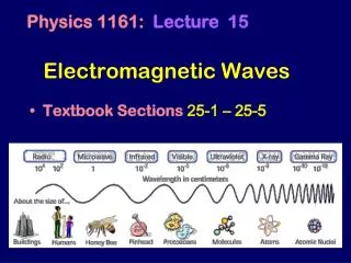
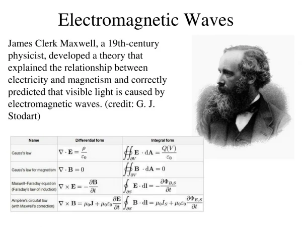
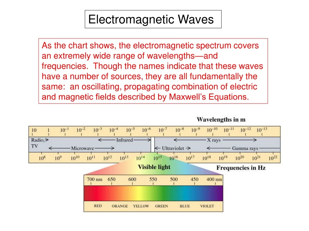
Electromagnetic Waves As the chart shows, the electromagnetic spectrum covers an extremely wide range of wavelengths—and frequencies. Though the names indicate that these waves have a number of sources, they are all fundamentally the same: an oscillating, propagating combination of electric and magnetic fields described by Maxwell’s Equations.
Mechanical waves Before studying electromagnetic waves, we’ll consider mechanical waves that we can see with our eyes, or hear with our ears. We shall see that many of the physical principles at work in these waves also apply to electromagnetic waves.
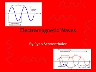
Transverse waves on a string As the top diagram on the previous slide showed, one form of wave that can be sent down a string is a “pulse” of arbitrary shape. But we are most interested in periodic waves, with a waveform that repeats after one “wavelength”, l [m]. And, in many cases we will be studying “sinusoidal”, or “harmonic” waves, that have a fixed frequency, f [Hz = cycles/s]. This picture shows one way to produce such a wave on a string. A mass attached to a spring is oscillating at its natural frequency f. If we tie a string to this mass, the waves traveling away from the mass will have the same frequency, f. That is, if we look at any location along the string we will see it moving up and down at f Hz. But what determines the wavelength l?? If the waves are moving away from the source slowly (rapidly), they will have a short (long) wavelength. So the speed of the wave, v [m/s], determines the wavelength. The relationship is very simple:
General characteristics of periodic waves The speed of the wave, v, is characteristic of the medium in which the wave propagates, and the parameters of that medium. For example, for a string, the speed of the wave depends on the tension in the string, T, and its mass per unit length, m. For a sinusoidal wave, the “waveform” will appear if we graph the wave as a function of position (left). The period, T, (the time for one cycle at any chosen position), will appear if we graph the wave as a function of time (right): In these graphs, “A” stands for the “amplitude” of the wave: its maximum excursion from zero. Notice that these graphs are of the form y = -A sin(ax) for the left graph, and y = A sin(bt)for the right graph. But… (1) What are a and bin terms of the parameters l,and f or T ? and (2) How do we incorporate the wave speed v??
Equations applying to all periodic waves Recapping, for all periodic waves, so far we have the following relationships: For the left-hand graph we can rewrite a in terms of wavelength: (Check by letting x be an integral number of wavelengths.) For the right-hand graph we can rewrite b in terms of period: (Check by letting t be an integral number of periods.) We have succeeded in relating the waveform and the temporal oscillations to wave parameters, but how do we describe a wave traveling at speed v? We put both factors into the argument of the sine function. How do we find the velocity of this wave? By seeing how the “zero-crossings” move with time. For example, let’s find the position of the zero for y = sin(0): This wave is traveling to the left with speed v!
Equations applying to all periodic waves… We just established that this equation describes a wave traveling to the left with speed . As you can quickly check, if we had put a minus sign between the terms, we would be describing a wave traveling to the right (in the +x direction). For convenience, we usually write these equations in terms of “angular quantities” so that the factors of 2p can be dropped. For the factor involving time, this should look very familiar: the angular frequency For the factor involving the spatial oscillations, or “waveform”: the “wave number” This is a new quantity, but it is just 2p times the number of wavelengths per meter. With these constants, we can write equations for traveling waves very simply! right with and and left
First look at an electromagnetic wave This is the waveform of an electromagnetic wave traveling in the +x direction with speed v = c = 2.99792458 x 10⁸ m/s. All electromagnetic waves travel at this speed—the “speed of light”—in a vacuum. Electromagnetic waves consist of an oscillating electric field, E, coupled to an oscillating magnetic field, B, with the same wavelength and frequency. These changing fields create and reinforce each other through the physical effects summarized in Faraday’s Law of Induction and the Ampere-Maxwell Law. There are no charges or currents present—only free, propagating fields. Discuss eqns We can describe this particular wave using the general equations from previous slides: and with and and
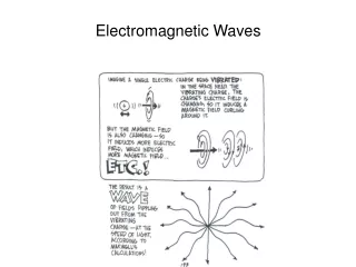
First look at an electromagnetic wave… Derivation of the wave equation is long, and hard to remember. So we’ll “cartoon” it. Faraday’s Law of Induction Ampere-Maxwell Law The light wave shown here is “linearly polarized in the y direction”. This means that its electric field oscillates in the y direction only. Because Eand B both oscillate perpendicular to the direction of motion, this is a transverse wave.But, in contrast to a wave on a string, there is no transverse displacement in y or z. This picture represents the electric and magnetic fields that would be measured along the x axis as the wave moves.
What is a “wave equation” ? A “wave equation” is a differential equation connecting the spatial shape of the wave to the time development of the wave, at a given location x and time t. As we’ll see, its solutions are the sinusoidal waves we’ve been discussing. For waves on a string: For E or B components of electromagnetic waves: Let’s illustrate this for Eyof the electromagnetic wave we’ve been studying: Yes, this satisfies the wave equation, and produces the correct velocity relationship. Similarly, so does Bi . If we put these into the wave equation for Eiand cancel –Emaxcos(kx – wt) we get:
Relative magnitudes of E and B in electromagnetic waves In many situations, electric and magnetics fields have different sources, and their magnitudes are not related in any fundamental way. But for electromagnetic waves in vacuum or in materials, Faraday’s Law and the Ampere-Maxwell Law force them to be in a certain ratio. The result in vacuum is, very simply: (32.4 in text)
Electromagnetic waves in materials Electromagnetic waves travel more slowly in materials than they do in vacuum. For visible light, we are most interested in transparent materials such as glasses, plastics, liquids (especially water), and gases. The ratio of the speed of light in vacuum to the speed in the given material, is called the “index of refraction”, n: The table at right lists the index of refraction for a number of common (and uncommon) materials. You can see the trend that the index of refraction rises with density. If we want to calculate the speed of light in these materials, we solve for v above: Fundamentally:
General wave properties again: Wave sources radiate power, as the waves carry away energy. 1D 2D For 2D systems, such as ripples on a pond, the intensity (energy density along the wave front) drops off as 1/r from the source. For perfect 1D systems, the energy put in by the source does not diminish with distance. 3D For 3D systems, such as point sources of light, the intensity (energy density per unit area in the wave front) drops off as 1/r2.
The power carried by a wave is proportional to A2 The upper graph is the sinusoidal wave picture we’ve seen before. The lower graph is the square of the upper one, multiplied by some additional factors, to give the power delivered by the wave as a function of time. Emax For a string, the equations for these graphs are: [W] For an electromagnetic wave (recall u): [W/m2] Power or intensity depend on the square of the amplitude of the wave! Notice that the intensity oscillates with time. But in most situations with electromagnetic waves, we don’t observe these rapid oscillations. (See next slide.)
Averaged quantities Quantities such as the power or intensity on the previous slide are called “instantaneous”, because at any given location they will fluctuate with time, proportional to the square of the sine function. But since the fluctuations are rapid, we are often more interested in “averaged” power or intensity. For a quantity that depends on the square of a sine or cosine the result is quite simple. The average of these functions over an integral number of cycles is half the maximum value. For the case of power, this is shown by the dashed line at Pav . This makes sense because the function is symmetric about the line: P spends the same time at a given value above the line as at a corresponding point at equal distance below the line. So from the instantaneous intensity on the previous slide, we can write down the average intensity in an electromagnetic wave: or, [W/m2]
Superposition of waves Using the example of pulses on a string, we can see that wave disturbances add (superpose). “Perfect” wave systems are linear. For electromagnetic waves, this is not surprising since we knew already that E and B obey the superposition principle, and electromagnetic waves are made from these fields. Sketch the case of two gaussian pulses (one inverted) passing through each other. After the string “goes flat”, how do they re-emerge?
Constructive and destructive interference in 1D Imagine that we have two sources creating two waves of the same frequency, traveling in the same direction, in the same region of space. The superposition principle say that we simply add them. What do we get? Destructive interference Constructive interference v In phase Out of phase Note: “Interference” means that they are “adding”. But it does not mean that they are “interacting” (changing each other’s wave properties)! What happens if they are traveling in opposite directions instead of the same direction?
EM waves interfering in 1D: some possibilities If we have two 1D waves interfering in some region, how do we write down the solution? Easy! Superposition tells us to just add the solutions. For the example of electromagnetic waves, we’ll look at the general solution for the total electric field. (The magnetic field solutions would look similar.) For the two cases plotted on the previous slide, we would choose the minus sign for travel to the right, and make the wave numbers and frequencies equal: Constructive interference,f=0: Zero if E1=E2 Destructive interference,f=180o: If they are equal magnitude, traveling in opposite directions, what do we get ? These waves are adding to create a “standing wave”, vibrating with amplitude E and frequency w. with zeroes (nodes) in fixed positions along the x-axis. More later!
Two-path interferometer. (Michelson inteferometer.) This is one way to create two light beams of the same frequency traveling in the same direction, with adjustable relative phase. The length of path 2 may be changed by moving mirror M2. The path length difference between routes 1 and 2 is Dd=2(L2 – L1), since each of the lengths is traveled twice in each path. When Dd is an integral number of wavelengths, nl, the light waves are in phase at the eye and bright spot is seen. For half-integral wavelengths, no light is seen along the line of the beam.
Constructive and destructive interference in 2D These are waves on the surface of water in a “ripple tank”. The drivers have small points touching the water surface, and all are operating at the same frequency. For one source we see a 2d wave traveling outward. For multiple sources, we see a complex pattern of constructive and destructive interference in 2D. Single source (half view) Three sources Two sources Imagine the patterns you would see in 3D!
Huygens’ principle Christiaan Huygens, 1629–1695 Christiaan Huygens was a mathematician, astronomer and physicist. The Huygens–Fresnel principle (named for Dutch physicist Christiaan Huygens, and French physicist Augustin-Jean Fresnel) is a method of analysis applied to problems of wave propagation. It recognizes that each point of an advancing wave front is in fact the center of a fresh disturbance and the source of a new train of waves; and that the advancing wave as a whole may be regarded as the sum of all the secondary waves arising from points in the medium already traversed. This view of wave propagation helps better understand a variety of wave phenomena, such as diffraction.
Huygens’ principle applied to a spherical wave in 3D Each point on an advancing wave front is a point source, or “wavelet”, which interferes constructively with other wavelets on the front to sustain the wave. Wave front at later time tB Wave front at time tA Point source on the wave front at time tA “Wavelet” from that point, at later time tB. (Small black arc.) This is an example of a “convex” wave front. Use Huygens’ principle to determine how a “concave” wave front would develop with time.
Far from a point source: “plane waves” This is another general property of waves. The further you get from the source, the more gradual the curvature of the wave front. In the “far field”, the wave fronts can be treated as planar. 2D ripple tank 3D Electromagnetic wave