Download

1 / 25
250 likes | 409 Views
Using Simulations to understand the Central Limit Theorem. Parameter : A number describing a characteristic of the population ( usually unknown ). The mean gas price of regular gasoline for all gas stations in Maryland . The mean gas price in Maryland is $______.

E N D
Parameter: A number describing a characteristic of the population (usually unknown) The mean gas price of regular gasoline for all gas stations in Maryland
The mean gas price in Maryland is $______ Statistic: A number describing a characteristic of a sample.
In Inferential Statisticswe use the value of a sample statistic to estimate a parameter value.
We want to estimate the mean height of MC students. The mean height of MC students is 64 inches
Will x-bar be equal to mu? What if we get another sample, will x-bar be the same? How much does x-bar vary from sample to sample? By how much will x-bar differ from mu? How do we investigate the behavior of x-bar?
Graph the x-bar distribution, describe the shape and find the mean and standard deviation
Simulation Rolling a fair die and recording the outcome randInt(1,6) Press MATH Go to PRB Select 5: randInt(1,6)
Rolling a die n times and finding the mean of the outcomes. Let n = 2 and think on the range of the x-bar distribution What if n is 10? Think on the range Mean(randInt(1,6,10) Press 2nd STAT[list] Right to MATH Select 3:mean( Press MATH Right to PRB 5:randInt(
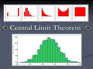
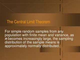
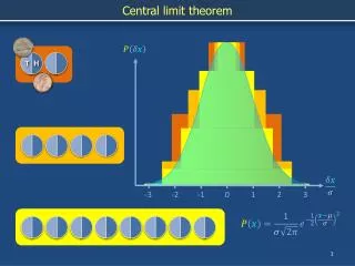
Rolling a die n times and finding the mean of the outcomes. The Central Limit Theorem in action
For the larger sample sizes, most of the x-bar values are quite close • to the mean of the parent population mu. • (Theoretical distribution in this case) • This is the effect of averaging • When n is small, a single unusual x value can result in an x-bar value far from the center • With a larger sample size, any unusual x values, when averaged • with the other sample values, still tend to yield an x-bar value close to mu. • AGAIN, an x-bar based on a large will tends to be closer to mu than will an x-bar based on a small sample. This is why the shape of the x-bar distribution becomes more bell shaped as the sample size gets larger.
The Central Limit Theorem in action Closing stock prices ($) Variability of sample means for samples of size 64 26 – 2.526 + 2.5 26 + 2*2.5 __|________|________|________X________|________|________|__ 18.5 21 23.5 26 28.5 31 33.5
Closing stock prices ($) Variability of sample means for samples of size 64 2.5% | 95% | 2.5% 26 – 2.5 26 + 2.5 26 + 2*2.5 __|________|________|________X________|________|________|__ 18.5 21 23.5 26 28.5 31 33.5 About 95% of samples of 64 closing stock prices have means that are within $5 of the population mean mu About 99.7% of samples of 64 closing stock prices have means that are within $7.50 of the population mean mu
We want to estimate the mean closing price of stocks by using a SRS of 64 stocks. Assume the standard deviation σ = $20. X ~Right Skewed (μ = ?, σ = 20) __|________|________|________X________|________|________|__ μ-7.5 μ-5 μ-2.5 μμ+2.5 μ+5 μ+7.5 We’ll be 95% confident that our estimate is within $5 from the population mean mu We’ll be 99.7% confident that our estimate is within $7.50 from the population mean mu
Simulation Roll a die 5 times and record the number of ONES obtained: randInt(1,6,5) Press MATH Go to PRB Select 5: randInt(1,6,5)
Roll a die 5 times, record the number of ONES obtained. Do the process n times and find the mean number of ONES obtained. The Central Limit Theorem in action