The basics of probability theory . Distribution o f variables, some important distributions
The basics of probability theory . Distribution o f variables, some important distributions. Random experiment. The outcome is not determined uniquely by the considered conditions.

The basics of probability theory . Distribution o f variables, some important distributions
E N D
Presentation Transcript
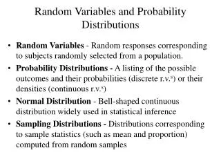
The basics of probability theory. Distribution of variables, some important distributions
Random experiment • The outcome is not determined uniquely by the considered conditions. • For example, tossing a coin, rolling a dice, measuring the concentration of a solution, measuring the body weight of an animal, etc. are experiments. • Every experiment has more, sometimes infinitely large outcomes Biostat 4.
Event: the result (or outcome) of an experiment • elementary events: the possible outcomes of an experiment. • composite event: it can be divided into sub-events. • Example. The experiment is rolling a dice. • Elementary events are 1,2,3,4,5,6. • Composite events: • E1={1,3,5} (the result is an odd number). • E2={2,4,6} (the result is an even number). • E3={5,6} (the result is greater than 4). • W={1,2,3,4,5,6} (the result is the certain event). Biostat 4.
Operations with events • The complementary event of an event A is the event which occurs whenever A fails. • Example: = ={2,4,6} • The sum of two events A and B is the event A+B which occurs if A or B occurs. • E1+E2={1,3,5}+{2,4,6}={1,2,3,4,5,6} • E1+E3={1,3,5}+{5,6}={1,3,5,6} • The product of two events A and B is the event AB which occurs if A and B occur. • E1·E2={1,3,5}·{2,4,6}= • E1·E3={1,3,5}·{5,6}={5} • If A ·B =, then we say that A and B are mutually exclusive events. Biostat 4.
The concept of probability Biostat 4.
The concept of probability • Lets repeat an experiment n times under the same conditions. In a large number of n experiments the event A is observed to occur k times (0 k n). • k : frequency of the occurrence of the event A. • k/n : relative frequency of the occurrence of the event A. 0 k/n 1 If n is large, k/n will approximate a given number. This number is called the probability of the occurrence of the event A and it is denoted by P(A). 0 P(A) 1 Biostat 4.
Example: the tossing of a (fair) coin k: number of „head”s n= 10 100 1000 10000 100000 k= 7 42 510 5005 49998 k/n= 0.7 0.42 0.51 0.5005 0.49998 P(„head”)=0.5 Biostat 4.
Probability facts • Any probability is a number between 0 and 1. • All possible outcomes together must have probability 1. • The probability of the complementary event of A is 1-P(A). Biostat 4.
Formula for the calculation of simple exact probabilities Biostat 4.
Rules of probability calculus • Assumption: all elementary events are equally probable Examples: • Rolling a dice. What is the probability that the dice shows 5? • If we let X represent the value of the outcome, then P(X=5)=1/6. • What is the probability that the dice shows an odd number? • P(odd)=1/2. Here F=3, T=6, so F/T=3/6=1/2. Biostat 4.
Population, sample Biostat 4.
Population, sample • Population: the entire group of individuals that we want information about. • Sample: a part of the population that we actually examine in order to get information • A simple random sample of size n consists of n individuals chosen from the population in such a way that every set of n individuals has an equal chance to be in the sample actually selected. Biostat 4.
Sample data set Questionnaire filled in by a group of pharmacy students Blood pressure of 20 healthy women … Population Pharmacy students Students Blood pressure of women (whoever) … Examples Biostat 4.
Bar chart of relative frequencies of a categorical variable Distribution of that variable in the population Sample Population (approximates)
Histogram of relative frequencies of a continuous variable Distribution of that variable in the population Sample Population (approximates)
Mean (x) Standard deviation (SD) Median Mean (unknown) Standard deviation (unknown) Median (unknown) Sample Population (approximates)
Random variables,probability distributions(distribution of the population) Biostat 4.
Random variables, probability distributions • A random variable is a variable whose value is a numerical outcome of a random phenomenon. • Notation: X, Y, .. • Examples • The experiment is tossing a coin. • X(H)=1 and X(T)=2 • Y(H)=-10 and Y(T)=10 • The experiment is rolling a dice. ={1,2,3,4,5,6}. Let define the X to be the number shown on the dice. Biostat 4.
Distribution of a discrete (categorical) random variable • A discrete random variable X has finite number of possible values • The probability distribution of X lists the values and their probabilities: Value of X: x1 x2 x3 … xn Probability: p1p2p3 … pn pi0, p1 + p2 +p3 … +pn =1 Biostat 4.
Examples • The experiment is rolling a dice. p1 =1/6, p2 =1/6,…, p6 =1/6 • The experiment is tossing a coin. p1 =0.5, p2 =0.5 Biostat 4.
Example: rolling two dices • Let random variable X be the sum of the two numbers shown on the two dices. • P(X=1)=0, (X=1 is impossible) • P(X=2)=1/36 (the only favourable event is (1,1), and the number of all possible event is 36. ) Biostat 4.
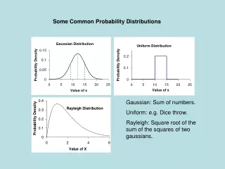
Uniform discrete distributions: all pi-s are equal Not uniform Biostat 4.
The binomial distribution • Let's consider an experiment Athat may have only two possible mutually exclusive outcomes (success, failure) • Let P(A)=p • We now repeat the experiment n times, let X denote the absolute frequency of the event A. • The probability that X will assume any given possible value k is expressed by the binomial formula Biostat 4.
Example In a certain population the occurrence of some disease is p=0.3. What is the probability that examining n=10 patients, there will be exactly k=4 diseased? According to the formula, P(X=4)=10!/(4!6!)(0.3)4(0.7)6=210 0.0081 0.117649= 0.200120949. Biostat 4.
Continuous random variable • A continuous random variable X has takes all values in an interval of numbers. • The probability distribution of Xis describedby a density curve. • The density curve • is on the above the horizontal axis, and • has area exactly 1 underneath it. • The probability of any event is the area under the density curve and above the values of X that make up the event. P(A) A Biostat 4.
P(A) A The density curve • The density curve is an idealized description of the overall pattern of a distribution that smoothes out the irregularities in the actual data. • The density curve • is on the above the horizontal axis, and • has area exactly 1 underneath it. • The area under the curve and above any range of values is the proportion of all observations that fall in that range. Biostat 4.
The density curve • The density curve • is on the above the horizontal axis: f(x) ≥0 • has area exactly 1 underneath it. ab • The area under the curve and above any range of values is the proportion of all observations that fall in that range. Biostat 4.
Special density curve:Normal distribution Biostat 4.
Special distribution of a continuous variable: The normal distribution • The normal curve was developed mathematically in 1733 by DeMoivre as an approximation to the binomial distribution. His paper was not discovered until 1924 by Karl Pearson. Laplace used the normal curve in 1783 to describe the distribution of errors. Subsequently, Gauss used the normal curve to analyze astronomical data in 1809. • The normal curve is often called the Gaussian distribution. • The term bell-shaped curve is often used in everyday usage. Biostat 4.
Special distribution of a continuous variable: The normal distribution N(,2) • The density curves are symmetric, single-peaked and bell-shaped • The 68-95-99.7 rule . In the normal distribution with mean and standard deviation : • 68% of the observations fall within of the mean • 95% of the observations fall within 2 of the mean • 99.7% of the observations fall within 3 of the mean Biostat 4.
Normal distributions N(, 2) N(0,1) N(1,1) , :parameters (a parameter is a number that describes the distribution) N(0,2) Biostat 4.
„Imagination” of the distribution given the sample mean and sample SD – supposing normal distribution • In the papers generally sample means and SD-s are published. We use these value to know the original distribution • For example, age in years: 55.2 15.7 39.5 70.9 68.26% of the data are supposed to be in this interval 95.44% of the data are supposed to be in the interval (23.8, 86.6) Biostat 4.
Stent length per lesion (mm): 18.8 10.5 Using these values as parameters, the „normal” distribution would be like this: The original distribution of stent length was probably skewed, or if the distribution was normal, there were negative values in the data set. Biostat 4.
Standard normal probabilities -1.96 1.96 0.025 0.95 0.025 Biostat 4.
The central limit theorem Biostat 4.
Distribution of sample meanshttp://onlinestatbook.com/stat_sim/sampling_dist/index.html Biostat 4.
The population is not normally distributed Biostat 4.
The central limit theorem • If the sample size n is large (say, at least 30), then the population of all possible sample means approximately has a normal distribution with mean µand standard deviation no matter what probability describes the population sampled Biostat 4.
Tha standard error of mean(SE or SEM) • is called the standard error of mean • Meaning: the dispersion of the sample means around the (unknown) population mean. Biostat 4.
Calculation of the standard error from the standard deviation when is unknown • Given x1,x2,x3,…,xnstatistical sample, the stadard error can be calculated by • It expresses the dispersion of the sample means around the (unknown) population mean. Biostat 4.
Review questions • What is the concept of probability? • What is the formula for computing simple exact probabilities? When can it be used? • What is the distribution of a discrete variable? • What are the properties of a discrete distribution? • What is the distribution of a continuous variable? • What are the properties of the density function? • What is the uniform distribution? • What is the binomial distribution? • What is the normal distribution? • Parameters of the normal distribution. • Properties of the normal distribution. Biostat 4.
Problems • If we roll a dice, there are 6 possible outcomes. If X represents the value of the outcome, find the following probabilities: a) P(X=1); b) P(X>1); c) P(1<X<4) • A fair coin is tossed twice. List the possible outcomes? What is the probability of getting two tails? • For a standard normal distribution, find the following probabilities using the standard normal table: • P(X<0)=…. • P(X>0)=….. • P(X<1)=…. • P(X>1)=….. • P(X<-1)=….. • P(-1<X<1)=……… Biostat 4.
Useful WEB pages • http://onlinestatbook.com/rvls/index.html • http://my.execpc.com/~helberg/statistics.html • http://www.regentsprep.org/Regents/math/algtrig/ATS2/NormalLesson.htm Biostat 4.