JGR-Oceans, October 2013 issue
240 likes | 434 Views
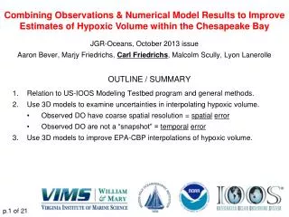
Combining Observations & Numerical Model Results to Improve Estimates of Hypoxic Volume w ithin the Chesapeake Bay. JGR-Oceans, October 2013 issue Aaron Bever , Marjy Friedrichs, Carl Friedrichs , Malcolm Scully, Lyon Lanerolle. OUTLINE / SUMMARY

JGR-Oceans, October 2013 issue
E N D
Presentation Transcript
Combining Observations & Numerical Model Results to Improve Estimates of Hypoxic Volume within the Chesapeake Bay JGR-Oceans, October 2013 issue Aaron Bever, Marjy Friedrichs, Carl Friedrichs, Malcolm Scully, Lyon Lanerolle • OUTLINE / SUMMARY • Relation to US-IOOS Modeling Testbed program and general methods. • Use 3D models to examine uncertainties in interpolating hypoxic volume. • Observed DO have coarse spatial resolution = spatialerror • Observed DO are not a “snapshot” = temporalerror • Use 3D models to improve EPA-CBP interpolations of hypoxic volume. p.1 of 21
Combining Observations & Numerical Model Results to Improve Estimates of Hypoxic Volume within the Chesapeake Bay • Relationship to US-IOOS Modeling Testbed: • Part of Coastal & Ocean Modeling Testbed (COMT) Project headed by Rick Luettich(UNC), funded by NOAA US-IOOS Office • COMT Mission: Accelerate the transition of scientific and technical advances from the modeling research community to improve federal agencies’ operational ocean products and services • Initial Phase: EstuarineHypoxia, Shelf Hypoxia and Coastal Inundation Modeling Testbeds; Cyber-infrastructure to advance interoperability and archiving p.2 of 21
Combining Observations & Numerical Model Results to Improve Estimates of Hypoxic Volume within the Chesapeake Bay General COMT Estuarine Hypoxia modeling methods: • Compare relative skill and strengths/weaknesses of various Chesapeake Bay models • Assess how model differences affect water quality simulations • Recommend improvements to agency operational products associated with managing hypoxia p.3 of 21
Five hydrodynamic models configured for the Bay TODAY’S TALK p.4 of 21
Five dissolved oxygen (DO) modelsconfigured for the Bay • ICM: EPA-CBP model; complex biology • BGC: NPZD-type biogeochemical model • 1eqn: Simple one equation respiration • (includes SOD) • 1term-DD: depth-dependent respiration • (not a function of x, y, temperature, nutrients…) • 1term: Constant net respiration • (not a function of x, y, temperature, nutrients OR depth…) p.5 of 21
Five dissolved oxygen (DO) modelsconfigured for the Bay • ICM: EPA-CBP model; complex biology • BGC: NPZD-type biogeochemical model • 1eqn: Simple one equation respiration • (includes SOD) • 1term-DD: depth-dependent respiration • (not a function of x, y, temperature, nutrients…) • 1term: Constant net respiration • (not a function of x, y, temperature, nutrients OR depth…) TODAY’S TALK p.5 of 21
Coupled hydrodynamic-DO models • Today’s talk = Four combinations: • CH3D + ICM EPA-CBP model • CBOFS + 1term • ChesROMS + 1term • ChesROMS + 1term+DD -- Physical models are similar, but grid resolution differs -- Biological/DO models differ dramatically -- All models run for 2004 and 2005 and compared to EPA Chesapeake Bay Program DO observations p.6 of 21
Model skill: Bottom DO Total RMSD2 = Bias2 + unbiased RMSD2 -- The models all have significant skill (normalized RSMD < 1) in reproducing observed bottom dissolved oxygen (DO). -- The four models all reproduce observations of bottom DO about equally well. -- Unlike observations, model output is continuous in space and time. -- So use the continuous model output to estimate uncertainties caused by CBP interpolations of discontinous observed data. p.7 of 21
Combining Observations & Numerical Model Results to Improve Estimates of Hypoxic Volume within the Chesapeake Bay JGR-Oceans, October 2013 issue Aaron Bever, Marjy Friedrichs, Carl Friedrichs, Malcolm Scully, Lyon Lanerolle • OUTLINE • Relation to US-IOOS Modeling Testbed program and general methods. • Use 3D models to examine uncertainties in interpolating hypoxic volume. • Observed DO have coarse spatial resolution = spatialerror • Observed DO are not a “snapshot” = temporalerror • Use 3D models to improve EPA-CBP interpolations of hypoxic volume. p.8 of 21
Four Types of Hypoxic Volume Estimates • Interpolation Method used for #1 - #3: • CBP Interpolator Tool • HV = DO < 2 mg/L • #1) Observations • Of 99 CBP stations (red dots), 30-65 are sampled each “cruise” • Each cruise takes 1 to 2 weeks • #2) Modeled Absolute Match: • Same 30-65 stations are “sampled” at same time/place as observations are available • #3) Modeled Spatial Match: • Same stations are “sampled” in space, but samples are taken synoptically (i.e., all at once in time) • #4) Integrated 3D Model: • Hypoxic volume is computed from integrating over all model grid cells (“CBP” = EPA Chesapeake Bay Program) p.9 of 21
Hypoxic Volume Estimates • When observations and model are interpolated in same way, the match is reasonably good CH3D-ICM = Absolute Match ChesROMS+1term Observations-derived p.10 of 21
Hypoxic Volume Estimates • When observations and model are interpolated in same way, the match is reasonably good • But interpolated HV underestimates actual HV for every cruise CH3D-ICM = Absolute Match CH3D-ICM ChesROMS+1term ChesROMS+1term Observations-derived Data-derived p.11 of 21
Hypoxic Volume Estimates • When observations and model are interpolated in same way, the match is reasonably good • But interpolated HV underestimates actual HV for every cruise • Much of this disparity could be due to temporal errors (red bars) CH3D-ICM ChesROMS+1term Observations-derived p.12 of 21
When observations and model are interpolated in same way, the match is reasonably good • But interpolated HV underestimates actual HV for every cruise • Much of this disparity could be due to temporal errors (red bars) • Same pattern across all 4 models for both 2004 & 2005 p.13 of 21
Spatial errors show interpolated HV is almost always too low (up to 5 km3) The temporal errors from non-synoptic sampling can be as large as spatial errors (~5 km3) Similar patterns across all 4 models for both 2004 & 2005 p.14 of 21
Combining Observations & Numerical Model Results to Improve Estimates of Hypoxic Volume within the Chesapeake Bay JGR-Oceans, October 2013 issue Aaron Bever, Marjy Friedrichs, Carl Friedrichs, Malcolm Scully, Lyon Lanerolle • OUTLINE • Relation to US-IOOS Modeling Testbed program and general methods. • Use 3D models to examine uncertainties in interpolating hypoxic volume. • Observed DO have coarse spatial resolution = spatialerror • Observed DO are not a “snapshot” = temporalerror • Use 3D models to improve EPA-CBP interpolations of hypoxic volume. p.15 of 21
Improving observation-derived hypoxic volumes Blue triangles = 13 selected CBP stations • Reduce Temporal errors: • Choose subset of 13 CBP stations • Routinely sampled within 2.3 days of each other • Characterized by high DO variability p.16 of 21
Improving observation-derived hypoxic volumes Blue triangles = 13 selected CBP stations • Reduce Temporal errors: • Choose subset of 13 CBP stations • Routinely sampled within 2.3 days of each other • Characterized by high DO variability But why 13 stations? p.16 of 21
Improving observation-derived hypoxic volumes Modeled Integrated 3D vs. Spatial Match for Different Station Sets p.17 of 21
Improving observation-derived hypoxic volumes • Reduce Spatial errors: • 1. For each model and each cruise, derive a correction factor as a function of interpolated HV that “corrects” this 13-station Spatial Match HV to equal the Integrated 3D HV. p.18 of 21
Improving observation-derived hypoxic volumes • Reduce Spatial errors: • 1. For each model and each cruise, derive a correction factor as a function of interpolated HV that “corrects” this 13-station Spatial Match HV to equal the Integrated 3D HV. • 2. Apply correction factor to HV time-series • 3. Scaling-corrected “interpolated” HV more accurately represents true HV Before Scaling After Scaling p.19 of 21
Interannual (1984-2012) corrected (i.e., scaled) time series of observed Hypoxic Volume • Time-series of corrected hypoxic volume for 1984-2012 are provided within JGR article (annual maximum HV, annual duration of HV, annual cumulative HV), and corrected HV for every CBP cruise is provided in JGR electronic supplement. p.20 of 21
Combining Observations & Numerical Model Results to Improve Estimates of Hypoxic Volume within the Chesapeake Bay Summary/Conclusions • Information from multiple models (2004-2005) has been used to assess uncertainties in present CBP interpolated hypoxic volume estimates • Temporal uncertainties: up to ~5 km3 • Spatial uncertainties: up to ~5 km3 • These are significant, given maximum HV is ~10-15 km3 • A method for correcting interpolated HV time series for temporal and spatial errors has been presented, based on the 3D structure of multiple model DO results • 13 stations (sample in 2 days) do as well for HV as 40-60 or more • Corrected HV for 1984-2012 are downloadable from JGR website p.21 of 21