Download
1 / 71
720 likes | 907 Views
FPGA Applications IEEE Micro Special Issue on Reconfigurable Computing Vol. 34, No.1, Jan.-Feb. 2014. Dr. Philip Brisk Department of Computer Science and Engineering University of California, Riverside CS 223. Guest Editors. Walid Najjar UCR. Paolo Ienne EPFL, Lausanne, Switzerland.

E N D
FPGA ApplicationsIEEE Micro Special Issue on Reconfigurable ComputingVol. 34, No.1, Jan.-Feb. 2014 Dr. Philip Brisk Department of Computer Science and Engineering University of California, Riverside CS 223
Guest Editors WalidNajjar UCR Paolo Ienne EPFL, Lausanne, Switzerland
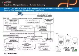
High-Speed Packet Processing Using Reconfigurable Computing Gordon Brebner and Weirong Jiang Xilinx, Inc.
Contributions • PX: a domain-specific language for packet-processing • PX-to-FPGA compiler • Evaluation of PX-designed high-performance reconfigurable computing architectures • Dynamic reprogramming of systems during live packet processing • Demonstrated implementations running at 100 Gbps and higher rates
PX Overview • Object-oriented semantics • Packet processing described as component objects • Communication between objects • Engine • Core packet processing functions • Parsing, editing, lookup, encryption, pattern matching, etc. • System • Collection of communicating engines and/or sub • Parsing, editing, lookup, encryption, pattern matching, etc.
Interface Objects • Packet • Communication of packets between components • Tuple • Communication of non-packet data between components
OpenFlow Packet Classification in PX Send packet to parser engine
OpenFlow Packet Classification in PX Parser engine extracts a tuple from the packet Send the tuple to the lookup engine for classification
OpenFlow Packet Classification in PX Obtain the classification response from the lookup engine Forward the response to the flowstream output interface
OpenFlow Packet Classification in PX Forward the packet (without modification) to the outstream output interface
PX Compilation Flow 100 Gbps : 512-bit datapath 10 Gbps : 64-bit datapath Faster to reconfigure the generated architecture than the FPGA itself (not always applicable)
OpenFlow Packet Parser (4 Stages) Allowable Packet Structures: (Ethernet, VLAN, IP, TCP/UDP) (Ethernet, IP, TCP/UDP) Stage 1: Ethernet Stage 2: VLAN or IP Stage 3: IP or TCP/UDP Stage 4: TCP/UDP or bypass
OpenFlow Packet Parser Max. number of stacked sections Max. packet size Structure of the tuple Ethernet header expected first Set relevant members in the tuple Being populated I/O interface Determine the type of the next section of the packet Determine how far to go in the packet to reach the next section
Three-stage Parser Pipeline • Internal units are customized based on PX requirements • Units are firmware-controlled • Specific actions can be altered (within reason) without reconfiguring the FPGA • e.g., add or remove section classes handled at that stage
OpenFlow Packet Parser Results Adjust throughput for wasted bits at the end of packets
Ternary Content Addressable Memory (TCAM) TCAM width and depth are configurable in PX X = Don’t Care http://thenetworksherpa.com/wp-content/uploads/2012/07/TCAM_2.png
TCAM Implementation in PX key length result bitwidth depth Set up TCAM access The parser (previous example) extracted the tuple Collect the result TCAM architecture is generated automatically as described by one of the authors’ previous papers
TCAM Parameterization • PX Description • Depth (N) • Width • Result width • Operational Properties • Number of rows (R) • Units per row (L) • Internal pipeline stages per unit (H) • Performance • Each unit handles N/(LR) TCAM units • Lookup latency is LH + 2 clock cycles • LH to process the row • 1 cycle for priority encoding • 1 cycle for registered output
Database Analytics: A Reconfigurable Computing Approach Bharat Sukhwani, Hong Min, Mathew Thoennes, ParijatDube, Bernard Brezzo, SamehAsaad, and Donna Eng. Dillenberger IBM T.J. Watson Research Center
Online Transaction Processing (OLTP) • Rows are compressed for storage and I/O savings • Rows are decompressed when issuing queries • Data pages are cached in a dedicated memory space called the buffer pool • I/O operations between buffer pool and disk are transparent • Data in the buffer pool is always up-to-date
Table Traversal • Indexing • Efficient for locating a small number of records • Scanning • Sift through the whole table • Used when a large number of records match the search criteria
Workflow • DBMS issues a command to the FPGA • Query specification and pointers to data • FPGA • Pulls pages from main memory • Parses pages to extract rows • Queries the rows • Writes qualifying queries back to main memory in database-formatted pages
FPGA Query Processing • Join and sort operations are not streaming • Data re-use is required • FPGA block RAM storage is limited • Perform predicate evaluation and projection before join and sort • Eliminate disqualified rows • Eliminate unneeded columns
Where is the Parallelism? • Multiple tiles process DB pages in parallel • Concurrently evaluate multiple records from a page within a tile • Concurrently evaluate multiple predicates against different columns within a row
Predicate Evaluation Stored predicate values Logical Operations (Depends on query) #PEs and reduction network size are configurable at synthesis time
Two-Phase Hash-Join • Stream the smaller join table through the FPGA • Hash the join columns to populate a bit vector • Store the full rows in off-chip DRAM • Join columns and row addresses are stored in the address table (BRAM) • Rows that hash to the same position are chained in the address table • Stream the second table through the FPGA • Hash rows to probe the bit vector (eliminate non-matching rows) • Matches issue reads from off-chip DRAM • Reduces off-chip accesses and stalls
Database Sort • Support long sort keys (tens of bytes) • Handle large payloads (rows) • Generate large sorted batches (millions of records) • Coloring bins keys into sorted batches https://en.wikipedia.org/wiki/Tournament_sort
CPU Savings Predicate Eval. Decompression + Predicate Eval.
Scaling Reverse Time Migration Performance Through Reconfigurable Dataflow Engines Haohan Fu1, Lin Gan1, Robert G Clapp2, Huabin Ruan1, Oliver Pell3, Oskar Mencer3, Michael Flynn2, Xiaomeng Huang1, and Guangwen Yang1 1Tsinghua University 2Stanford University 3Maxeler Technologies
Migration (Geology) https://upload.wikimedia.org/wikipedia/commons/3/38/GraphicalMigration.jpg
Reverse Time Migration (RTM) • Imaging algorithm • Used for oil and gas exploration • Computationally demanding
RTM Pseudocode Iterations over shots (sources) are independent and easy to parallelize Add the recorded source signal to the corresponding location Iterate over time-steps, and 3D grids Propagate source wave fields from time 0 to nt - 1 Boundary conditions Iterate over time-steps, and 3D grids Add the recorded receiver signal to the corresponding location Propagate receiver wave fields from time nt - 1 to 0 Cross-correlate the source and receiver wave field at the same time step to accumulate the result Boundary conditions
RTM Computational Challenges • Cross-correlate source and receiver signals • Source/receiver wave signals are computed in different directions in time • The size of a source wave field for one time-step can be 0.5 to 4 GB • Checkpointing: store source wave field and certain time steps and recompute the remaining steps when needed • Memory access pattern • Neighboring points may be distant in the memory space • High cache miss rate (when the domain is large)
Java-like HDL / MaxCompilerStencil Example Automated construction of a window buffer that covers different points needed by the stencile Data type: no reason that all floating-point data must be 32- or 64-bit IEEE compliant (float/double)
Performance Tuning • Optimization strategies • Algorithmic requirements • Hardware resource limits • Balance resource utilization so that none becomes a bottleneck • LUTs • DSP Blocks • block RAMs • I/O bandwidth
Algorithm Optimization • Goal: • Avoid data transfer required to checkpoint source wave fields • Strategies: • Add randomness to the boundary region • Make computation of source wave fields reversible
Custom BRAM Buffers 37 pt. Star Stencil on a MAX3 DFE • 24 concurrent pipelines at 125 MHz • Concurrent access to 37 points per cycle • Internal memory bandwidth of 426 Gbytes/sec
More Parallelism • Process multiple points concurrently • Demands more I/O • Cascade multiple time steps in a deep pipeline • Demands more buffers
Number Representation • 32-bit floating-point was default • Convert many variables to 24-bit fixed-point • Smaller pipelines => MORE pipelines Floating-point • 16,943 LUTs • 23,735 flip-flops • 24 DSP48Es Fixed-point • 3,385 LUTs • 3,718 flip-flops • 12 DSP48Es
Hardware Decompression • I/O is a bottleneck • Compress data off-chip • Decompress on the fly • Higher I/O bandwidth • Wave field data • Must be read and written many times • Lossy compression acceptable • 16-bit storage of 32-bit data • Velocity data and read-only Earth model parameters • Store values in a ROM • Create a table of indices into the ROM • Decompression requires ~1300 LUTs and ~1200 flip-flops
Performance Model • Memory bandwidth constraint # points processed in parallel compression ratio # bytes per point memory bandwidth frequency • Resource constraint (details omitted)