Download
1 / 23
230 likes | 246 Views
Explore examples for biomass burning, LULUCF in Finland, and the conservativeness approach applied to the Democratic Republic of Congo (DRC) with a focus on estimating uncertainties in environmental assessments. Learn methods, data, and analysis techniques used in these cases.

E N D
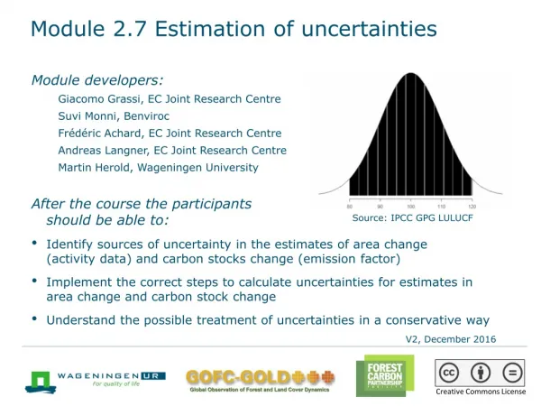
Module 2.7 Estimation of uncertainties Module developers: Giacomo Grassi , Joint Research Centre Suvi Monni, Benviroc Frédéric Achard, Joint Research Centre Andreas Langner, Joint Research Centre Martin Herold, Wageningen University Country examples: • Biomass burning • LULUCF in Finland • Appling the conservativeness approach to the DRC example (matrix approach); this example also relates to Module 3.3 Source: IPCC GPG LULUCF V1, May 2015 Creative Commons License
Example 1: Biomass burning (1/2) • This country example shows a combination of uncertainties for non-CO2 emissions from biomass burning for an Annex I party. • Note that no uncertainty is assumed for GWP values. • The table below shows the data used in the calculations.
Example 2: LULUCF in Finland (1/3)* • For its GHG inventory, . • T. * Synthesis from the National Inventory Report of Finland (Statistics Finland 2013). Table: Inventory uncertainties
Example 2: LULUCF in Finland (2/3) • Forforest land remaining forest land, uncertainty analysis is done by pools: living biomass, mineral, and organic soils. Both sampling uncertainty of national forest inventory (NFI) and model uncertainty (used for reporting) are considered. • gain-loss method is applied, which requires data regarding increment and losses: • Uncertainty (U%) includes sampling of volume increment (4-13%), BCEF (0.5-2.5%),
Example 2: LULUCF in Finland (3/3) • Conversion to/from forest land and related KP activities: estimation of C stock change in all pools is done by: AD x EF. • Uncertainty of AD due to sampling was estimated from NFI: • Because of small land areas involved, a high sampling error is reported:e.g., U% for deforestation is 30% • U% in the increment of living biomass and in the mineral and organic soil emission factors is based on expert judgement. • For emissions from soils under conversions of forest land to cropland and grassland, preliminary estimates are 60–150%.
Example 3: Appling the conservativeness approach to the Democratic Republic of Congo (DRC) example (matrix approach) (1/14) • (This example also relates to exercise 4 and Module 3.3) • IPCC basics to estimate forest C stock changes • Emissions = activity data (AD) x emission factor (EF) • Six land uses: forest land, cropland, grassland, wetlands, settlements, other lands • Methods to estimate C stock changes: • Gain-loss: growth minusharvest minusother losses (all tiers) • Stock change: difference of C stock over time (only Tiers 2–3)IPCC would require Tier 2/3 methods for EF in "Key Categories" (likely including deforestation and degradation in most cases), but most developing countries are not ready yet for Tier 2/3.
Example 3: REDD+ matrix (2/14) How would REDD+ activities fit into IPCC land uses? Stock change method: C before minusC after Gain-loss: growth minusharvest minusother losses Difficult to get data IPCC (very uncertain) FAOSTAT: very difficult to get the right data! Overall, unlikely to estimate C stock changes from degradation with tier 1
Example 3: REDD+ matrix (3/14) Don’t forget degradation! Estimates of carbon emissions from degradation (expressed as an additional percentage to the emissions from deforestation)
Example 3: REDD+ matrix (4/14) Modified IPCC land transition matrix (REDD+ matrix) Stock change method: C before – C after Gain-loss: growth – harvest – other losses
Example 3: REDD+ matrix (5/14) How to identify non–intact forests? • Among different possible approaches, forest edges may be used as a simple and pragmatic proxy to identify non–intact areas (boundary forests), or at least may be a first step to be complemented by other more accurate approaches (i.e., high-resolution remote sensing). • The underlying assumption is that forests that are sufficiently remote from nonforested areas (i.e., at a certain distance from roads, navigable waters, crops, grasslands, mines, etc.) are protected against significant anthropogenic degradation.
Example 3: REDD+ matrix (6/14) Example of identification of boundary forests • Input: binary forest maps using the methodology of FAO Remote Sensing Survey • Intensified sampling 60x60 m² • Treatment: morphological spatial pattern analysis (MSPA) • Biome specific: rainforest in Congo Basin (Edge size=500m) • Could as well be called exposed, potentially degraded, managed,or simply other forests.
Example 3: REDD+ matrix (7/14) Case study in DRC Area transition matrices for a biome: Congo rainforests (ha 000s) NFL = natural forest land; BFL = boundary forest; OL = other land.
Example 3: REDD+ matrix (8/14) Area-based hypothetical reference level NFL = natural forest land; BFL = boundary forest; OL = other land
Example 3: REDD+ matrix (9/14) Estimating C stock changes for REDD activities • Once the transition matrix for AD is done, each AD will need to be multiplied by the relevant EF to get C stock change for each REDD+ activity: • For natural forest, Tier 1 EF are available from IPCC • For boundary forests, data may be taken from the literature (or a crude assumption of half of C stock of NFL may be considered) • Uncertainties values need to be associated with each EF. • The proposed approach requires that the same Tier 1 EF (stratified by forest and climate type) be used in both reference level (RL) and in the accounting period. This means that the errors of EF in the RL and accounting period are fully correlated.
Example 3: REDD+ matrix (10/14) NFL = natural/intact forest land; BFL = boundary forest; OL = other land. (a) Assuming these values of biomass C stocks: NFL, 155 tC/ha (IPCC 2006); EFL, NFL/2 (or 50% degradation on average in exposed forests); OL, 5 tC/ha. (b) Calculated as the difference in area (actual minus RL) x the C stock change.
Example 3: REDD+ matrix (11/14) Taking uncertainties into account Assume that estimates for (accounting period minus RL) obtained with adequate methods for AD but not for EF (Tier 1) When the uncertainties above are combined, total uncertainty of the emission reduction (19,4 Mt C) becomes >100% (95%CI) How to deal with the fact that this country used Tier 1 (highly uncertain) EF for a key category? see next slides
Example 3: REDD+ matrix (12/14) As part of the Kyoto Protocol review process, UNFCCC has approved conservativeness factors linked to specific uncertainty ranges. Essentially, these factors use the 50% confidence interval.
Example 3: REDD+ matrix (13/14) 95% confidence interval 50% confidence interval Lower bound of 50% CI (≈14MtC) In this example, by discounting the emissions reduction by about 30% (following the approach of KP review), the risk of overestimating the reduction of emissions is significantly reduced.
Example 3: REDD+ matrix (14/14) • In conclusion, the REDD+ matrix may allow one to estimate C stock change from deforestation/degradation based on IPCC Tier 1. • The application of a conservative discount to address the high uncertainty of Tier 1–based estimates increases the credibility of any possible claim of result-based payment. • The simplicity and cost-effectiveness of this approach may allow: • Broadening the participation to REDD+, allowing those countries with limited forest monitoring capacity to join • Increasing the credibility of emission reductions estimated with Tier 1, while maintaining strong incentives for further increasing the accuracy of the estimates, i.e., to move to higher tiers
Recommended modules as follow-up • Module 2.8 to learn more about the role of evolving technologies for monitoring of forest area changes and changes in forest carbon stocks • Modules 3.1 to 3.3 to proceed with REDD+ assessment and reporting
References • Achard, F., Eva, H. D., Mayaux, P., Stibig, H.-J. and Belward, A., 2004. Improved estimates of net carbon emissions from land cover change in the tropics for the 1990s. Glob. Biogeochem. Cycles 18, GB2008. • Asner, G. P., Knapp, D. E., Broadbent, E. N., Oliveira, P. J. C., Keller, M. and Silva, J. N., 2005. Selective logging in the Brazilian Amazon. Science 310, 480–2. • Bucki, M., D. Cuypers, P. Mayaux, F. Achard, C. Estreguil, and G. Grassi.2012. “Assessing REDD+ Performance of Countries with Low Monitoring Capacities: The Matrix Approach.” Environmental Research Letters 7 (1) 014031. • Gaston, G., Brown, S., Lorenzini, M. and Singh, K. D., 1998. State and change in carbon pools in the forests of tropical Africa. Glob. Change Biol. 4, 97–114. • Houghton, R. A., 2003. Revised estimates of the annual net flux of carbon to the atmosphere from changes in land use and land management 1850–2000. Tellus, B, 55, 378–90.
Houghton, R. A. and Hackler, J. L., 1999. Emissions of carbon from forestry and land-use change in tropical Asia. Glob. Change Biol. 5, 481–92. • IPCC (Intergovernmental Panel on Climate Change). 2000. Good Practice Guidance and Uncertainty Management in National Greenhouse Gas Inventories. (Often IPCC GPG.) Geneva, Switzerland: IPCC. http://www.ipcc-nggip.iges.or.jp/public/gp/english/. • IPCC, 2003. 2003 Good Practice Guidance for Land Use, Land-Use Change and Forestry, Prepared by the National Greenhouse Gas Inventories Programme, Penman, J., Gytarsky, M., Hiraishi, T., Krug, T., Kruger, D., Pipatti, R., Buendia, L., Miwa, K., Ngara, T., Tanabe, K., Wagner, F. (eds.). Published: IGES, Japan. http://www.ipcc-nggip.iges.or.jp/public/gpglulucf/gpglulucf.html (Often referred to as IPCC GPG) • Statistics Finland. 2013. Greenhouse Gas Emissions in Finland, 1990–2011: National Inventory Report under the UNFCCC and the Kyoto Protocol. Helsinki: StatisticsFinland. http://unfccc.int/national_reports/annex_i_ghg_inventories/national_inventories_submissions/items/7383.php.