Objectives: Elements of a Discrete Model Evaluation Decoding Dynamic Programming

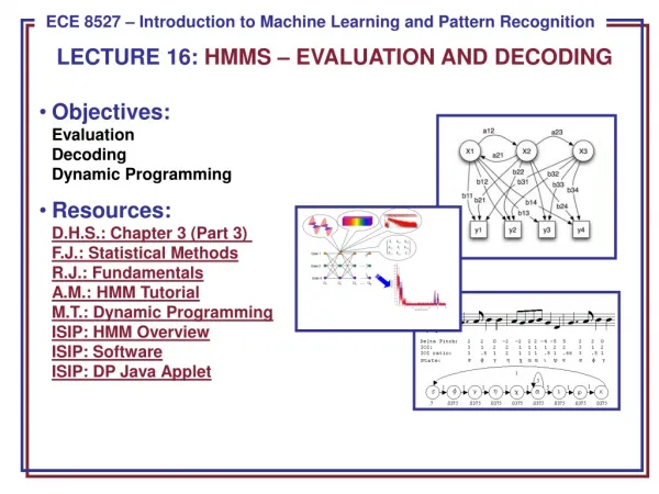
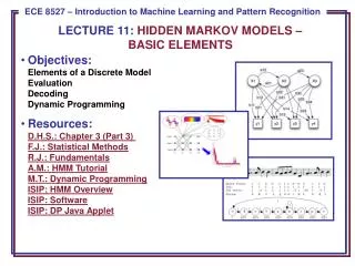
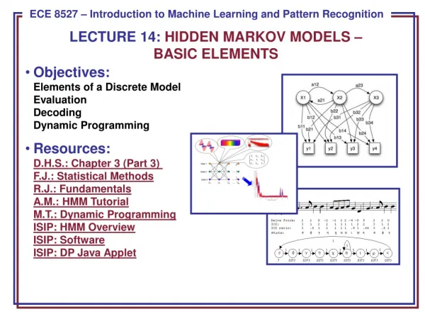
1. LECTURE 14: HIDDEN MARKOV MODELS –BASIC ELEMENTS • Objectives:Elements of a Discrete ModelEvaluationDecodingDynamic Programming • Resources:D.H.S.: Chapter 3 (Part 3) F.J.: Statistical MethodsR.J.: FundamentalsA.M.: HMM TutorialM.T.: Dynamic ProgrammingISIP: HMM OverviewISIP: SoftwareISIP: DP Java Applet

2. Introduction To Hidden Markov Models

3. Introduction To Hidden Markov Models (Cont.)

4. Introduction To Hidden Markov Models (Cont.)

5. Motivation • Thus far we have dealt with parameter estimation for the static pattern classification problem: estimating the parameters of class-conditional densities needed to make a single decision. • Many problems have an inherent temporal dimension – the vectors of interest come from a time series that unfolds as a function of time. Modeling temporal relationships between these vectors is an important part of the problem. • Markov models are a popular way to model such signals. There are many generalizations of these approaches, including Markov Random Fields and Bayesian Networks. • First-order Markov processes are very effective because they are sufficiently powerful and computationally efficient. • Higher-order Markov processes can be represented using first-order processes • Markov models are very attractive because of their ability to automatically learn underlying structure. Often this structure has relevance to the pattern recognition problem (e.g., the states represents physical attributes of the system that generated the data).

6. Discrete Hidden Markov Models • Elements of the model: • c states: • M output symbols: • c x c transition probabilities: • Note that the transition probabilities only depend on the previous state and the current state (hence , this is a first-order Markov process). • T x M output probabilities: • Initial state distribution:

7. More Definitions and Comments • The state and output probability distributions must sum to 1: • A Markov model is called ergodic if every one of the states has a nonzero probability of occurring given some starting state. • A Markov model is called a hidden Markov model (HMM) if the output symbols cannot be observed directly (e.g, correspond to a state) and can only be observed through a second stochastic process. HMMs are often referred to as a doubly stochastic system or model because state transitions and outputs are modeled as stochastic processes. • There are three fundamental problems associated with HMMs: • Evaluation: How do we efficiently compute the probability that a particular sequences of states was observed? • Decoding: What is the most likely sequences of hidden states that produced an observed sequence? • Learning: How do we estimate the parameters of the model?

8. Problem No. 1: Evaluation • The probability that we output a symbol at a particular time can also be easily computed: • Note that the probability of being in any state at time t is easily computed: • But these computations, which are of complexity O(cTT), where T is the length of the sequence), are prohibitive for even the simplest of models (e.g., c=10 and T=20 requires 1021 calculations). • We can calculate this recursively by exploiting the first-order property of the process, and noting that the probability of being in a state at time t is easily computed by summing all possible paths from previous states.

9. Summary • Formally introduced a hidden Markov model. • Described three fundamental problems (evaluation, decoding, and training). • Derived general properties of the model. • Remaining issues: • Introduce the Forward Algorithm as a fast way to do evaluation. • Introduce the Viterbi Algorithm as a reasonable way to do decoding. • Introduce dynamic programming using a string matching example. • Derive the reestimation equations using the EM Theorem so we can guarantee convergence. • Generalize the output distribution to a continuous distribution using a Gaussian mixture model.