Download
1 / 27
270 likes | 432 Views
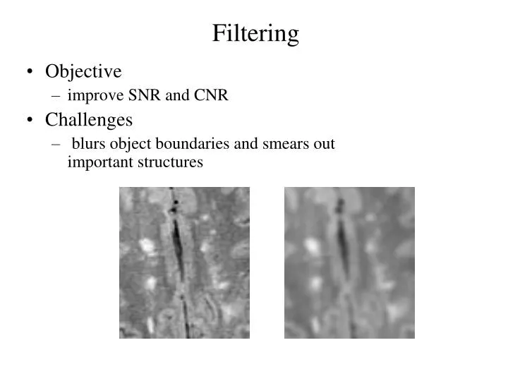
Filtering. Objective improve SNR and CNR Challenges blurs object boundaries and smears out important structures. Averaging using rotating mask. Consider each image pixel (i,j). Calculate dispersion in the mask for all possible mask rotations about (i,j).

E N D
Filtering • Objective • improve SNR and CNR • Challenges • blurs object boundaries and smears out important structures
Averaging using rotating mask • Consider each image pixel (i,j). Calculate dispersion in the mask for all possible mask rotations about (i,j). • Choose the mask with minimum dispersion. • Assign to the pixel (i,j) in the output image the average brightness in the chosen mask.
Anisotropic diffusive filtering • An iterative process in which intensity diffusion V takes place between adjacent spels in a nonlinear fashion with gradients F as follows: V = GF, where G is diffusion conductance
Diffusion • A diffusion process can be defined using the divergence operator “div” on a vector field. A mathematical formulation of the diffusion process on a vector field V at a point c
Mathematical formulation • D(c,d): the unit vector for c toward d • Intensity gradient at l-th iteration:
Continued… • Diffusion conductance function: • Diffusion flow
Continued … • Iterative diffusion process • Diffusion constant • Diffusion constant used here
MS 2D Examples Original MR image VOI from original image Anisotropic diffusion
MS 3D Examples Original MR image VOI from the original image Anisotropic diffusion
MS 2D Examples Original MR image VOI from original image Anisotropic diffusion Scale-based anisotropic diffusion
MS 3D Examples Anisotropic diffusion Original MR image VOI from the original image Scale-based anisotropic diffusion
original aniso. diff. s-scale t-scale Results
original aniso. diff. s-scale t-scale Zoomed Display
Canny’s edge detection • The detection criterion expresses the fact that important edges should not be missed and that there should be no spurious responses • The localization criterion minimizes the distance between the actual and the located edge position • The response criterion minimizes multiple response to a single edge
Scale in edge detection • Scale is a resolution or a range of resolution needed to provide a sufficient yet compact representation of the object or a target information • In a Gaussian smoothing or edge detection kernel the parameter σ resembles with scale
Canny’s edge localization • It seeks out zero-crossings of • In one-dimension a closed form solution may be found using calculus of variation. • In two or higher dimension, the best solution is obtained by a numerical optimization, called non-maximal suppression, that essentially seeks for the best solution for
Non-maximal suppression • Quantize edge directions eight ways according to 8-connectivity • For each pixel with non zero edge magnitude, inspect the two adjacent pixels indicated by the direction of its edge • If the magnitude of either of these two exceeds that of the pixel under inspection, mark it for deletion • When all pixels have been inspected, re-scan the image and erase to zero all edge data marked for deletion
Hysteresis to filter output of an edge operator • Mark all edges with magnitude greater than tH as correct • Scan all pixels with edge magnitude in the range [tL,tH] • If such a pixel is adjacent to another already marked as an edge, then mark it too. • Repeat from step 2 until stability
Canny’s edge detector • Convolve an image f with a Gaussian of scale σ • Localize edge points using the Non-Maximal Suppression algorithm • Compute edge magnitude of the edge at each locations • Apply the Hysteresis algorithm to filter edge locations eliminating spurious responses • Repeat steps (1) through (5) for ascending values of scales σ of a range [σmin, σmax] • Aggregate the edge information at different scale using feature synthesis
Examples LoG DoG Roberts Sobel Prewitt
Examples σ=1 σ=2 σ=3
Parametric edge detection • Facet model: a piecewise continuous function representing the intensity in the neighborhood of a pixel, e.g., a bi-cubic faced model
Parametric edge detection • Model parameters may be computed using a least-squares method with singular value decomposition • Facet model is computationally expensive but give more accurate localization of edges with sub-pixel accuracy • Haralick and Shairo shown that for a 5x5 facet model, the parameters may be directly computed using ten 5x5 kernels