Download

1 / 40
400 likes | 499 Views
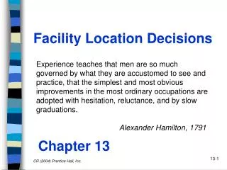
Facility Location Decisions. Experience teaches that men are so much governed by what they are accustomed to see and practice, that the simplest and most obvious improvements in the most ordinary occupations are adopted with hesitation, reluctance, and by slow graduations.

E N D
Facility Location Decisions Experience teaches that men are so much governed by what they are accustomed to see and practice, that the simplest and most obvious improvements in the most ordinary occupations are adopted with hesitation, reluctance, and by slow graduations. Alexander Hamilton, 1791 Chapter 13 CR (2004) Prentice Hall, Inc.
Inventory Strategy Inventory Strategy • • Forecasting Forecasting Transport Strategy Transport Strategy • • Inventory decisions Inventory decisions • • Transport fundamentals Transport fundamentals • • Purchasing and supply Purchasing and supply • • Transport decisions Transport decisions Customer Customer scheduling decisions scheduling decisions service goals service goals • • Storage fundamentals Storage fundamentals ORGANIZING ORGANIZING • • The product The product CONTROLLING CONTROLLING • • Storage decisions Storage decisions PLANNING PLANNING • • Logistics service Logistics service • • Ord Ord . proc. & info. sys. . proc. & info. sys. Location Strategy Location Strategy Location decisions Location decisions • • • • The network planning process The network planning process Facility Location in Location Strategy CR (2004) Prentice Hall, Inc.
Location Overview • What's located? • Sourcing points • Plants • Vendors • Ports • Intermediate points • Warehouses • Terminals • Public facilities (fire, police, and ambulance stations) • Service centers • Sink points • Retail outlets • Customers/Users CR (2004) Prentice Hall, Inc.
Location Overview (Cont’d) • Key Questions • How many facilities should there be? • Where should they be located? • What size should they be? • Why Location is Important • Gives structure to the network • Significantly affects inventory and transportation costs • Impacts on the level of customer service to be achieved CR (2004) Prentice Hall, Inc.
Location Overview (Cont’d) • Methods of Solution • Single warehouse location • Graphic • Grid, or center-of-gravity, approach • Multiple warehouse location • Simulation • Optimization • Heuristics CR (2004) Prentice Hall, Inc.
Nature of Location Analysis Manufacturing (plants & warehouses) Decisions are driven by economics. Relevant costs such as transportation, inventory carrying, labor, and taxes are traded off against each other to find good locations. Retail Decisions are driven by revenue. Traffic flow and resulting revenue are primary location factors, cost is considered after revenue. Service Decisions are driven by service factors. Response time, accessibility, and availability are key dimensions for locating in the service industry. CR (2004) Prentice Hall, Inc.
Weber’s Classification of Industries CR (2004) Prentice Hall, Inc.
Agglomeration Based on the observation that the output of one industry is the input of another. Customers for an industry’s products are the workers of those industries. Hence, suppliers, manufacturers, and customers group together, especially where transportation costs are high. Historically, the growth of the auto industry showed this pattern. Today, the electronics industry (silicon valley) has a similar pattern although it is less obvious since the product value is high and transportation costs are a small portion of total product price. CR (2004) Prentice Hall, Inc.
COG Method • Method appraisal • A continuous location method • Locates on the basis of transportation costs alone • The COG method involves • Determining the volumes by source and destination point • Determining the transportation costs based on $/unit/mi. • Overlaying a grid to determine the coordinates of source and/or destination points • Finding the weighted center of gravity for the graph CR (2004) Prentice Hall, Inc.
COG Method (Cont’d) where Vi = volume flowing from (to) point I Ri = transportation rate to ship Vi from (to) point i Xi,Yi = coordinate points for point i = coordinate points for facility to be located CR (2004) Prentice Hall, Inc.
Annual Rate, Point Prod- volume, $/ cwt/ i ucts Location cwt. mi. X Y i i 1 S A Seattle 8,000 0.02 0.6 7.3 1 2 S B Atlanta 10,000 0.02 8.6 3.0 2 3 H A & B Los 5,000 0.05 2.0 3.0 1 Angeles 4 H A & B Dallas 3,000 0.05 5.5 2.4 2 5 H A & B Chicago 4,000 0.05 7.9 5.5 3 6 H A & B New York 6,000 0.05 10.6 5.2 4 COG Method (Cont’d) Example Suppose a regional medical warehouse is to be established to serve several Veterans Administration hospitals throughout the country. The supplies originate at S1and S2 and are destined for hospitals at H1 through H4. The relative locations are shown on the map grid. Other data are: Note rate is a per mile cost CR (2004) Prentice Hall, Inc.
COG Method (Cont’d) Map scaling factor, K CR (2004) Prentice Hall, Inc.
i X Y V R V R V R X V R Y i i i i i i i i i i i i 1 0.6 7.3 8,000 0.02 160 96 1,168 2 8.6 3.0 10,000 0.02 200 1,720 600 3 2.0 3.0 5,000 0.05 250 500 750 4 5.5 2.4 3,000 0.05 150 825 360 5 7.9 5.5 4,000 0.05 200 1,580 1,100 6 10.6 5.2 6,000 0.05 300 3,180 1,560 1,260 7,901 5,538 COG Method (Cont’d) Solve the COG equations in table form CR (2004) Prentice Hall, Inc.
X Y COG Method (Cont’d) Now, = 7,901/1,260 = 6.27 = 5,538/1,260 = 4.40 This is approximately Columbia, MO. The total cost for this location is found by: where K is the map scaling factor to convert coordinates into miles. CR (2004) Prentice Hall, Inc.
COG Method (Cont’d) COG CR (2004) Prentice Hall, Inc.
Calculate total cost at COG i Xi Yi Vi Ri TC 1 0.6 7.3 8,000 0.02 509,482 2 8.6 3.0 10,000 0.02 271,825 3 2.0 3.0 5,000 0.05 561,706 4 5.5 2.4 3,000 0.05 160,733 5 7.9 5.5 4,000 0.05 196,644 6 10.6 5.2 6,000 0.05 660,492 COG Method (Cont’d) 2,360,882 Total CR (2004) Prentice Hall, Inc.
Note The center-of-gravity method does not necessarily give optimal answers, but will give good answers if there are a large numbers of points in the problem (>30) and the volume for any one point is not a high proportion of the total volume. However, optimal locations can be found by the exact center of gravity method. å å V R X /d V R Y /d n n i i i i i i i i = = X , Y i i å å V R /d V R /d i i i i i i i i where n n = - + - 2 2 d (X X ) (Y Y ) i i i and n is the iteration number. COG Method (Cont’d) CR (2004) Prentice Hall, Inc.
COG Method (Cont’d) Solution procedure for exact COG • Solve for COG • Using find di • Re-solve for using exact formulation • Use revised to find revised di • Repeat steps 3 through 5 until there is no change in • Calculate total costs using final coordinates CR (2004) Prentice Hall, Inc.
Multiple Location Methods • A more complex problem that most firms have. • It involves trading off the following costs: Transportation inbound to and outbound from the facilities - Storage and handling costs - Inventory carrying costs - Production/purchase costs - Facility fixed costs - • Subject to: Customer service constraints - Facility capacity restrictions - • Mathematical methods are popular for this type of problem that: Search for the best combination of facilities to minimize - costs Do so within a reasonable computational time - Do not require enormous amounts of data for the analysis - CR (2004) Prentice Hall, Inc.
Total cost Warehouse Cost fixed Inventory carrying and warehousing Production/purchase and order processing Inbound and outbound transportation 0 0 Number of warehouses Location Cost Trade-Offs CR (2004) Prentice Hall, Inc.
Multiple COG • Formulated as basic COG model • Can search for the best locations for a selected number of sites. • Fixed costs and inventory consolidation effects are handled outside of the model. • A multiple COG procedure • Rank demand points from highest to lowest volume • Use the M largest as initial facility locations and assign remaining demand centers to these locations • Compute the COG of the M locations • Reassign all demand centers to the M COGs on the basis of proximity • Recompute the COGs and repeat the demand center assignments, stopping this iterative process when there is no further change in the assignments or COGs CR (2004) Prentice Hall, Inc.
Examples of Practical COG Model Use • Location of truck maintenance terminals • Location of public facilities such as offices, and police and fire stations • Location of medical facilities • Location of most any facility where transportation cost (rather than inventory carrying cost and facility fixed cost) is the driving factor in location • As a suggestor of sites for further evaluation CR (2004) Prentice Hall, Inc.
A method used commercially - Has good problem scope - Can be implemented on a PC - Running times may be long and memory requirements substantial Handles fixed costs well - Nonlinear inventory costs are not well - handled • A linear programming-like solution procedure can be used (MIPROG in LOGWARE) Mixed Integer Programming CR (2004) Prentice Hall, Inc.
Example The database for the illustrated problem is prepared as file ILP02.DAT in MIPROG. The form is dictated by the problem formulation in the technical supplement of the location chapter. The solution is to open only one warehouse (W2) with resulting costs of: Category Cost Production $1,020,000 Transportation 1,220,000 Warehouse handling 310,000 Warehouse fixed 500,000 Total $3,050,000 MIP (Cont’d) CR (2004) Prentice Hall, Inc.
The situation MIP (Cont’d) A Multiple Product Network Design Problem
Guided Linear Programming for the best locations. Searches A typical problem is shown in the next figure and can be configured as a transportation problem of linear programming in terms of its variable costs. · per - unit The inventory and warehouse fixed costs are computed as costs, bu t this depends on the warehouse throughput. They are placed along with the variable costs in the linear programming problem. · The linear programming problem is solved. This gives revised demand assignments to warehouses. Some may have no throughput an d are closed. · Fixed costs and inventory carrying costs are recomputed based on revised warehouse throughputs. · When there is no change in the solution from one iteration to the next, STOP. CR (2004) Prentice Hall, Inc.
Guided Linear Programming (Cont’d) The situation CR (2004) Prentice Hall, Inc.
Guided Linear Programming (Cont’d) Example Use data from the network figure. · Allocate the fixed costs. Assume initially that each warehouse handles the · entire volume . Hence, Warehouse 1 100,000/200,000 = $0.50/cwt. Warehouse 2 400,000/200,000 = $2.00/cwt. Allocate inventory carrying costs. Assume that throughput for each product is · equally divided between warehouses. Total customer demand Each warehouse 0.7 100{[200,000/2 ) ]/(200,000/2)} = $3.2 No. of whses Build the cost matrix for the transportation problem of LP. Note its special · structure. 13-38 CR (2004) Prentice Hall, Inc.
Matrix of Cell Costs and Solution Values for the First Iteration in the Example Problem Warehouses Customers Plant & warehouse capacities W W C C C 2 1 2 3 1 a b 4 9 99 99 99 60,000 60,000 P 1 Plants 8 6 99 99 99 c 140,000 999,999 P 2 d 0 99 9.7 8.7 10.7 W 60,000 60,000 1 Warehouses e b 99 0 8.2 7.2 8.2 c 50,000 999,999 W 40,000 50,000 2 Warehouse capacity & customer c demand 60,000 999,999 50,000 100,000 50,000 13-39
Ware- Per-unit Fixed Cost, Per-Unit Inventory Carrying Cost, house $/cwt. $/cwt. 0.7 W $100,000/60,000 cwt. $100(60,000 cwt .) /60,000 cwt. 1 = 1.67 = 3.69 0.7 W $400,000/140,000 cwt. $100(140,000 cwt .) /140,000 cwt. 2 = 2.86 = 2.86 Place these per-unit costs along with transportation costs in the · transportation matrix. The portion of the matrix that is revised is: C C C 1 2 3 a W 11.36 10.36 12.36 1 b W 8.72 7.72 8.72 2 a 2 + 4 + 1.67 + 3.69 = 11.36 b Guided Linear Programming (Cont’d) Solve as an LP problem, transportation type. Note the results in the · solution matrix. Recompute the per-unit fixed and inventory costs from the first solution · results as follows. 1 + 2 + 3.57 + 2.86 = 9.43 13-40 CR (2004) Prentice Hall, Inc.
Warehouse 1 Warehouse 2 Cost type 0 cwt. 200,000 cwt. Production $0 200,000 4 = $800,000 ´ Inbound transportation 0 200,000 2 = 400,000 ´ Outbound transportation 50,000 2 = 100,000 ´ 100,000 1 = 100,000 ´ 0 50,000 2 = 100,000 ´ Fixed 0 400,000 0.7 Inventory carrying 0 100(200,000) = 513,714 Handling 0 200,000 1 = 200,000 ´ Subtotal $0 $2,613,714 Total $2,613,714 Guided Linear Programming (Cont’d)
Location by Simulation • Can include more variables than typical algorithmic methods • Cost representations can be precise so problem can be more accurately described than with most algorithmic methods • Mathematical optimization usually is not guaranteed, although heuristics can be included to guide solution process toward satisfactory solutions • Data requirements can be extensive • Has limited use in practice CR (2004) Prentice Hall, Inc.
Shycon/Maffei Simulation CR (2004) Prentice Hall, Inc.
Commercial Models for Location • Features • Includes most relevant location costs • Constrains to specified capacity and customer service levels • Replicates the cost of specified designs • Handles multiple locations over multiple echelons • Handles multiple product categories • Searches for the best network design CR (2004) Prentice Hall, Inc.
Commercial Models (Cont’d) 13-45 CR (2004) Prentice Hall, Inc.
Commercial Models (Cont’d) 13-46 CR (2004) Prentice Hall, Inc.
· The general long-range nature of the location problem - Network configurations are not implemented immediately - There are fixed charges associated with moving to a new configuration · We seek to find a set of network configurations that minimizes the present value over the planning horizon Retail Location · Contrasts with plant and warehouse location. - Revenue rather than cost driven - Factors other than costs such as parking, nearness to competitive outlets, and nearness to customers are dominant Methods · Weighted checklist - Good where many subjective factors are involved - Quantifies the comparison among alternate locations Dynamic Location CR (2004) Prentice Hall, Inc.
A Hypothetical Weighted Factor Checklist for a Retail Location Example (1) (2) ´ (3)=(1) (2) Factor Weight Factor Score Weighted a b (1 to 10) Location Factors (1 to 10) Score 8 Proximity to competing stores 5 40 5 Space rent/lease 15 3 considerations 8 Parking space 10 80 7 Proximity to complementary 56 8 stores 6 Modernity of store space 9 54 9 Customer accessibility 8 72 3 Local taxes 2 6 3 Community service 4 12 8 Proximity to major 56 7 transportation arteries Total index 391 13-48 CR (2004) Prentice Hall, Inc.