Download
1 / 47
470 likes | 663 Views
A ggregate D emand. Simulated AD. AE = [ W + Y e – PL – r – mpc ∙ T + I + G + X ] + { mpc – mpm } Y Y = [ W + Y e – PL – r – mpc ∙ T + I + G + X ] + { mpc – mpm } Y PL = [ W + Y e – r – mpc ∙ T + I + G + X ] + { mpc – mpm } Y – 1 Y

E N D
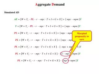
Aggregate Demand Simulated AD AE = [W + Ye – PL – r – mpc∙ T + I + G + X]+ {mpc– mpm}Y Y = [W + Ye – PL – r – mpc∙ T + I + G + X]+ {mpc– mpm}Y PL = [W + Ye – r – mpc∙ T + I + G + X]+ {mpc– mpm}Y – 1Y PL = [W + Ye – r – mpc∙ T + I + G + X]+ {mpc– mpm – 1}Y PL = [W + Ye – r – mpc∙ T + I + G + X]– {–mpc+ mpm + 1}Y PL = [W + Ye – r – mpc∙ T + I + G + X]– {1 – mpc+ mpm}Y PL = [W + Ye – r – mpc∙ T + I + G + X]– {mps+ mpm}Y Marginal propensity to save Marginal propensity to save
Aggregate Demand Simulated AD AE = [W + Ye – PL – r – mpc∙ T + I + G + X]+ {mpc– mpm}Y Y = [W + Ye – PL – r – mpc∙ T + I + G + X]+ {mpc– mpm}Y PL = [W + Ye – r – mpc∙ T + I + G + X]+ {mpc– mpm}Y – 1Y PL = [W + Ye – r – mpc∙ T + I + G + X]+ {mpc– mpm – 1}Y PL = [W + Ye – r – mpc∙ T + I + G + X]– {–mpc+ mpm + 1}Y PL = [W + Ye – r – mpc∙ T + I + G + X]– {1 – mpc+ mpm}Y PL = [W + Ye – r – mpc∙ T + I + G + X]– {mps+ mpm}Y
Aggregate Demand Simulated AD • Example:In addition to W = 5, Ye = 7, PL = 8, r = 2, mpc = 0.75, and T = 3, assume, investment expenditures total $1 trillion (I = 1), government expenditures total $3.5 trillion (G = 3.5), exports total $0.5 trillion (X = 0.5) with mpm= 0.25. Derive the AE equation. • First, ignore the fact that PL = 8 because AD isthe relationship between real GDP and PL • PL = [W + Ye – r – mpc∙ T + I + G + X]– {mps+ mpm}∙ Y
Aggregate Demand Simulated AD • Example:In addition to W = 5, Ye = 7, PL = 8, r = 2, mpc = 0.75, and T = 3, assume, investment expenditures total $1 trillion (I = 1), government expenditures total $3.5 trillion (G = 3.5), exports total $0.5 trillion (X = 0.5) with mpm= 0.25. Derive the AE equation. • First, ignore the fact that PL = 8 because AD isthe relationship between real GDP and PL • PL = [ 5 + Ye – r – mpc∙ T + I + G + X]– {mps+ mpm}∙ Y
Aggregate Demand Simulated AD • Example: In addition to W = 5, Ye = 7, PL = 8, r = 2, mpc = 0.75, and T = 3, assume, investment expenditures total $1 trillion (I = 1), government expenditures total $3.5 trillion (G = 3.5), exports total $0.5 trillion (X = 0.5) with mpm= 0.25. Derive the AE equation. • First, ignore the fact that PL = 8 because AD isthe relationship between real GDP and PL • PL = [ 5 + 7 – r – mpc∙ T + I + G + X]– {mps+ mpm}∙ Y
Aggregate Demand Simulated AD • Example:In addition to W = 5, Ye = 7, PL = 8, r = 2, mpc = 0.75, and T = 3, assume, investment expenditures total $1 trillion (I = 1), government expenditures total $3.5 trillion (G = 3.5), exports total $0.5 trillion (X = 0.5) with mpm= 0.25. Derive the AE equation. • First, ignore the fact that PL = 8 because AD isthe relationship between real GDP and PL • PL = [ 5 + 7 – 2 – mpc∙ T + I + G + X]– {mps+ mpm}∙ Y
Aggregate Demand Simulated AD • Example:In addition to W = 5, Ye = 7, PL = 8, r = 2, mpc = 0.75, and T = 3, assume, investment expenditures total $1 trillion (I = 1), government expenditures total $3.5 trillion (G = 3.5), exports total $0.5 trillion (X = 0.5) with mpm= 0.25. Derive the AE equation. • First, ignore the fact that PL = 8 because AD isthe relationship between real GDP and PL • PL = [ 5 + 7 – 2 – 0.75∙ T + I + G + X]– {0.25+ mpm}∙ Y
Aggregate Demand Simulated AD • Example:In addition to W = 5, Ye = 7, PL = 8, r = 2, mpc = 0.75, and T = 3, assume, investment expenditures total $1 trillion (I = 1), government expenditures total $3.5 trillion (G = 3.5), exports total $0.5 trillion (X = 0.5) with mpm= 0.25. Derive the AE equation. • First, ignore the fact that PL = 8 because AD isthe relationship between real GDP and PL • PL = [ 5 + 7 – 2 – 0.75∙ 3 + I + G + X]– {0.25+ mpm}∙ Y
Aggregate Demand Simulated AD • Example:In addition to W = 5, Ye = 7, PL = 8, r = 2, mpc = 0.75, and T = 3, assume, investment expenditures total $1 trillion (I = 1), government expenditures total $3.5 trillion (G = 3.5), exports total $0.5 trillion (X = 0.5) with mpm= 0.25. Derive the AE equation. • First, ignore the fact that PL = 8 because AD isthe relationship between real GDP and PL • PL = [ 5 + 7 – 2 – 0.75∙ 3 + 1 + G + X]– {0.25+ mpm}∙ Y
Aggregate Demand Simulated AD • Example:In addition to W = 5, Ye = 7, PL = 8, r = 2, mpc = 0.75, and T = 3, assume, investment expenditures total $1 trillion (I = 1), government expenditures total $3.5 trillion (G = 3.5), exports total $0.5 trillion (X = 0.5) with mpm= 0.25. Derive the AE equation. • First, ignore the fact that PL = 8 because AD isthe relationship between real GDP and PL • PL = [ 5 + 7 – 2 – 0.75∙ 3 + 1 + 3.5 + X]– {0.25+ mpm}∙ Y
Aggregate Demand Simulated AD • Example:In addition to W = 5, Ye = 7, PL = 8, r = 2, mpc = 0.75, and T = 3, assume, investment expenditures total $1 trillion (I = 1), government expenditures total $3.5 trillion (G = 3.5), exports total $0.5 trillion (X = 0.5) with mpm= 0.25. Derive the AE equation. • First, ignore the fact that PL = 8 because AD isthe relationship between real GDP and PL • PL = [ 5 + 7 – 2 – 0.75∙ 3 + 1 + 3.5 + 0.5]– {0.25+ mpm}∙ Y
Aggregate Demand Simulated AD • Example:In addition to W = 5, Ye = 7, PL = 8, r = 2, mpc = 0.75, and T = 3, assume, investment expenditures total $1 trillion (I = 1), government expenditures total $3.5 trillion (G = 3.5), exports total $0.5 trillion (X = 0.5) with mpm= 0.25. Derive the AE equation. • First, ignore the fact that PL = 8 because AD isthe relationship between real GDP and PL • PL = [ 5 + 7 – 2 – 0.75∙ 3 + 1 + 3.5 + 0.5]– {0.25+ 0.25}∙ Y • PL = 12.75 – 0.5Y
Aggregate Demand Simulated AD • Example: • PL = 12.75 – 0.5Y • By assumption, aggregate planned expenditure equals real GDP (Y = AE). • Recall that in the AE model, Y = 9.5 when PL = 8 at the Keynesian equilibrium point. PL 12.75 8 AD 0 9.5 Y
Aggregate Demand Simulated AD • Example: (continued): With real GDP equal to 9.5 trillion dollars, show what happens if • consumer wealth rises by 0.5 trillion dollars • expected future income increases by 0.5 trillion dollars • investment expenditure falls by 0.5 trillion dollars • exports rise to 1 trillion dollars • real rate of interestincreases by 0.5 pct. points • tax revenue is cut by 0.5 trillion dollars. Compute the tax cut multiplier. Compute the budget balance. • government expenditure is raised by 0.5 trillion dollars. Compute the government expenditure multiplier. Compute the budget balance. What is monetary policy, and who conducts it? What is fiscal policy, and who conducts it?
Long Run Aggregate Supply Simulated LRAS • Example: Suppose the economy’s production function shows the volume of output that can be produced by its labor force of size L given levels of K units of capital, R units of resources and Z percent of the knowledge/talent that is contained in the universe. Suppose resources, capital, & technology/talent are currently at R = 0.4 (trillion dollars of land, oil, coal, natural gas…), K = 2.5 (trillion dollars of machines, roads, networks…) and z = 1 (percent of all knowledge in the universe is known on Earth). • What is the economy’s short-run production function?
Long Run Aggregate Supply Simulated LRAS • Example (continued): 2. Graph the economy’s short-run production function L
Long Run Aggregate Supply Simulated LRAS • Example (continued): 3. Suppose there are 9 million workers that are frictionally or structurally unemployed, and 135 million of the 144 million in the labor force are employed. Compute u, un, uc, real GDP, and Yp. 12 144 L
Long Run Aggregate Supply Simulated LRAS • Example (continued): 4. Graph LRAS. LRAS PL 30 20 10 0 Y 12
Long Run Aggregate Supply Simulated LRAS • Example (continued): With the labor force equal to 144 million workers, show what happens if • Resources rises by 0.5 trillion dollars • Physical capital increases by 0.5 trillion dollars • The number of laborers falls by 12 million • Nominal wage rates rise by 1 thousand dollars • Nominal prices of other inputs increases by 1 thousand dollars • Supply side taxes are cut by 1 percentage point. What is monetary policy, and who conducts it? What is fiscal policy, and who conducts it?
Short Run Aggregate Supply SRAS is the relationship between the quantity of real GDP supplied and PL when all other influences on production plans remain the same • The SRAS curve is positively sloped (b) • Firms maximize profits. If prices increase while all other costs are constant, production rises because it is more profitable. Firm supply, industry supply and SRAS slope up. • Alternatively, when PL rises with constant wages, real wages falls, employment rises, and quantity of real GDP supplied rises. • Shifters of SRAS are contained in its intercept: • The money wage rate changes (w). • The money prices of other resources change (p). • Government changes supply-side taxes (t) • Factors that change Yp • Simulated SRAS has a slope of 1: PL = [ w + p + t – b·Yp ] + b·Y
Short Run Aggregate Supply Simulated SRAS • Example: In addition to R = 0.4 (trillion dollars of land…), K =2.5 (trillion dollars of machines…), Z = 1 (percent of all knowledge is known to man), Un = 9 (million frictionally or structurally unemployed workers), E = 135 (million), and L = 144 (million), suppose nominal wages are 2.25 (thousand dollars per month), the nominal price of other production factors is 0.75 (thousand dollars per month), the supply-side tax rate is 5 (percent), and slope is 1. 1. Graph the potential GDP you computed in part (3) with AD Yp = 12 PL = [ w + p + t – b·Yp ] + b·Y
Short Run Aggregate Supply Simulated SRAS • Example: In addition to R = 0.4 (trillion dollars of land…), K =2.5 (trillion dollars of machines…), Z = 1 (percent of all knowledge is known to man), Un = 9 (million frictionally or structurally unemployed workers), E = 135 (million), and L = 144 (million), suppose nominal wages are 2.25 (thousand dollars per month), the nominal price of other production factors is 0.75 (thousand dollars per month), the supply-side tax rate is 5 (percent), and slope is 1. 1. Graph the potential GDP you computed in part (3) with AD Yp = 12 PL = [ w + p+ t – 12 ] + Y
Short Run Aggregate Supply Simulated SRAS • Example: In addition to R = 0.4 (trillion dollars of land…), K =2.5 (trillion dollars of machines…), Z = 1 (percent of all knowledge is known to man), Un = 9 (million frictionally or structurally unemployed workers), E = 135 (million), and L = 144 (million), suppose nominal wages are 2.25 (thousand dollars per month), the nominal price of other production factors is 0.75 (thousand dollars per month), the supply-side tax rate is 5 (percent), and slope is 1. 1. Graph the potential GDP you computed in part (3) with AD Yp = 12 PL = [ 2.25 + p+ t – 12 ] + Y
Short Run Aggregate Supply Simulated SRAS • Example: In addition to R = 0.4 (trillion dollars of land…), K =2.5 (trillion dollars of machines…), Z = 1 (percent of all knowledge is known to man), Un = 9 (million frictionally or structurally unemployed workers), E = 135 (million), and L = 144 (million), suppose nominal wages are 2.25 (thousand dollars per month), the nominal price of other production factors is 0.75 (thousand dollars per month), the supply-side tax rate is 5 (percent), and slope is 1. 1. Graph the potential GDP you computed in part (3) with AD Yp = 12 PL = [ 2.25 + 0.75 + t – 12 ] + Y
Short Run Aggregate Supply Simulated SRAS • Example: In addition to R = 0.4 (trillion dollars of land…), K =2.5 (trillion dollars of machines…), Z = 1 (percent of all knowledge is known to man), Un = 9 (million frictionally or structurally unemployed workers), E = 135 (million), and L = 144 (million), suppose nominal wages are 2.25 (thousand dollars per month), the nominal price of other production factors is 0.75 (thousand dollars per month), the supply-side tax rate is 5 (percent), and slope is 1. 1. Graph the potential GDP you computed in part (3) with AD Yp = 12 PL = [ 2.25 + 0.75 + 5 – 12 ] + Y
Short Run Aggregate Supply Simulated SRAS • Example: In addition to R = 0.4 (trillion dollars of land…), K =2.5 (trillion dollars of machines…), Z = 1 (percent of all knowledge is known to man), Un = 9 (million frictionally or structurally unemployed workers), E = 135 (million), and L = 144 (million), suppose nominal wages are 2.25 (thousand dollars per month), the nominal price of other production factors is 0.75 (thousand dollars per month), the supply-side tax rate is 5 (percent), and slope is 1. 1. Graph the potential GDP you computed in part (3) with AD Yp = 12 PL = -4 + Y
Short Run Aggregate Supply Simulated SRAS • Example (continued): 2. Graph SRAS PL SRAS 8 12 Y -4
Short Run Aggregate Supply Simulated SRAS • Example (continued): 3. Graph SRAS and LRAS PL LRAS SRAS 8 12 Y -4
Short Run Aggregate Supply Simulated SRAS • Example (continued): 4. Suppose wages fall by 1 thousand dollars per month. PL LRAS PL = [ 2.25 + 0.75 + 5 – 12 ] + Y PL = -5 + Y SRAS SRAS’ 8 12 Y 13.2 -4 -5
Short Run Aggregate Supply Simulated SRAS • Example (continued): 5. Suppose technology increases by 0.1 percentage points. PL LRAS’ LRAS SRAS 144 Yp= 13.2 (trillion $) 8 12 Y 13.2 -4
Short Run Aggregate Supply Simulated SRAS • Example (continued): 5. Suppose technology increases by 0.1 percentage points. PL LRAS’ LRAS SRAS SRAS’ Yp= 13.2 (trillion $) 8 PL = [2.25 + 0.75 + 5 – 12 ] + Y PL = -5.2 + Y 12 Y 13.2 -4 -5.2
Short Run Aggregate Supply Simulated SRAS • Example (continued):With the labor force equal to 144 million workers, show what happens if • Resources rises by 0.5 trillion dollars • Physical capital increases by 0.5 trillion dollars • The number of laborers falls by 12 million • Nominal wage rates rise by 1 thousand dollars • Nominal prices of other inputs increases by 1 thousand dollars • Supply side taxes are cut by 1 percentage point. What is monetary policy, and who conducts it? What is fiscal policy, and who conducts it?
Aggregate Market Model Equilibrium • Example (continued): 1. Graph LRAS, SRAS and AD Yp= 12 PL = 12.75 – 0.5Y PL = -4 + Y PL LRAS 12.75 SRAS 8 6.75 AD 12 Y -4
Aggregate Market Model Equilibrium • Example (continued): 1. Graph LRAS, SRAS and AD Yp= 12 PL = 12.75 – 0.5Y PL = -4 + Y PL LRAS 12.75 SRAS 7.167 AD 12 Y -4 11.167
Aggregate Market Model Equilibrium • Example (continued): 1. Graph LRAS, SRAS and AD Yp= 12 PL = 12.75 – 0.5Y PL = -4 + Y PL LRAS 12.75 SRAS Recessionary gap 7.167 AD 12 Y -4 11.167
Aggregate Market Model Equilibrium • Example (continued): 1. Graph LRAS, SRAS and AD Yp= 12 PL = 12.75 – 0.5Y PL = -4 + Y PL = [w + p + t – Yp] + Y PL LRAS Factories, resources, and workers are not being fully utilized. Unemployment is higher than its natural rate. The surplus of workers bids down wages, which lowers SRAS until the gap is closed. 12.75 SRAS Recessionary gap 7.167 6.75 AD 12 Y -4 11.167
Aggregate Market Model Equilibrium • Example (continued): 1. Graph LRAS, SRAS and AD Yp= 12 PL = 12.75 – 0.5Y PL = -4 + Y Allowing the gap to close on its on is called laissez faire policy. Recessionary gaps tend to close slowly. The federal min wage was enacted in 1938. John L. Lewis (UMW, CIO, USWA) organized millions of workers in the 1930s. TANF, SNAP… PL LRAS 12.75 SRAS Recessionary gap 7.167 6.75 AD 12 Y 11.167
Aggregate Market Model Equilibrium • Example (continued): 1. Graph LRAS, SRAS and AD Yp= 12 PL = 12.75 – 0.5Y PL = -4 + Y Deflation sounds good because lower prices raise purchasing power. However, deflation causes hardships for those whose net worth is mostly held in illiquid assets (homes). Deflation amplifies debt since it was incurred when wages were higher. The same payment with a lower wage reduces purchasing power. Deflation amplifies a loan's interest rate. PL LRAS 12.75 SRAS Recessionary gap 7.167 6.75 AD 12 Y 11.167
Aggregate Market Model Equilibrium • Example (continued): 1. Graph LRAS, SRAS and AD Yp= 12 PL = 12.75 – 0.5Y PL = -4 + Y PL = [5 + 7 – 2 – 0.75∙3 + 1 + 3.5 + 0.5] –{0.25+ 0.25}∙Y PL = 14 – 0.5Y 4.75 Raising G by $1.25t, shifts AD, and closes the recessionary gap. Real GDP increases by $0.833t. The G-multiplier is 0.833 1.25 or 0.67 The budget deficit increases from $0.5t to $1.75t. The price level rises by 11.6% PL LRAS 12.75 SRAS 8 Recessionary gap 7.167 AD 12 Y 11.167
Aggregate Market Model Equilibrium • Example (continued): 1. Graph LRAS, SRAS and AD Yp= 12 PL = 12.75 – 0.5Y PL = -4 + Y PL = [5 + 7 – 2 – 0.75∙ 3 + 1 + 3.5 + 0.5] –{0.25+ 0.25}∙Y PL = 14 – 0.5Y 1.33 Cutting T by $1.667t, shifts AD, and closes the recessionary gap. Real GDP increases by $0.833t. The T-cut-mult is 0.833 1.667 or 0.5 The budget deficit increases from $0.5t to $2.167t. The price level rises by 11.6% PL LRAS 12.75 SRAS 8 Recessionary gap 7.167 AD 12 Y 11.167
Aggregate Market Model Equilibrium • Example (continued): 2. Graph LRAS, SRAS and AD Yp= 12 PL = 14 – 0.5Y PL = -6 + Y PL LRAS 14 SRAS 7.167 AD 12 Y -6 13.333
Aggregate Market Model Equilibrium • Example (continued): 2. Graph LRAS, SRAS and AD Yp= 12 PL = 14 – 0.5Y PL = -6 + Y PL LRAS 14 SRAS Inflationary gap 7.167 AD 12 Y -6 13.333
Aggregate Market Model Equilibrium • Example (continued): 2. Graph LRAS, SRAS and AD Yp= 12 PL = 14 – 0.5Y PL = -6 + Y PL = [w + p + t – Yp ] + Y PL Workers work overtime and/or more than one job, and firms compete for scarce labor. Unemployment is lower than its natural rate. For these reasons, there are upward pressures on wages. This raises SRAS until the gap is closed. LRAS 14 SRAS 8 Inflationary gap 7.167 AD 12 Y -6 13.333
Aggregate Market Model Equilibrium • Example (continued): 2. Graph LRAS, SRAS and AD Yp= 12 PL = 14 – 0.5Y PL = -6 + Y PL Allowing gaps to close on their own via changes in wages is a laissez faire policy. Inflationary gaps can close fast. The inflation redistributes income from those on fixed incomes to those with variable income. Governments have used inflation as a tax to avoid cutting G or increasing T. LRAS 14 SRAS 8 7.167 AD 12 Y 11.167
Aggregate Market Model Equilibrium • Example (continued): 3. Graph LRAS, SRAS and AD Yp= 12 PL = 14 – 0.5Y PL = -6 + Y PL = [W+ Ye– r –mpc∙T+ I+ G+ X]–{0.25+ 0.25}∙Y PL LRAS SRAS Induced Inflationary gap 9 8 AD 12 Y 13
Aggregate Market Model Equilibrium • Example (continued): 3. Graph LRAS, SRAS and AD Yp= 12 PL = 14 – 0.5Y PL = -6 + Y PL = [w + p + t – Yp] + Y PL LRAS If nothing is done to combat this stimulus, w rises as labor markets tighten. SRAS Induced Inflationary gap 9 8 AD 12 Y 13
Aggregate Market Model Equilibrium • Example (continued): 3. Graph LRAS, SRAS and AD Yp= 12 PL = 14 – 0.5Y PL = -6 + Y PL = [w + p + t – Yp] + Y PL LRAS If nothing is done to combat this stimulus, w rises as labor markets tighten. Hence, the increase in GDP was only temporary. Prices soar even more. SRAS 9.5 Induced Inflationary gap 9 8 AD 12 Y 13