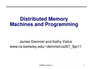
Distributed Memory Computers and Programming
This document presents a comprehensive overview of distributed memory architectures and programming paradigms. It examines various topologies such as linear, ring, mesh, and hypercubical networks, discussing their properties, cost models, and implications for communication efficiency. The historical evolution of distributed systems is explored, highlighting the transition from early queue-based systems to modern direct memory access mechanisms. Key concepts such as latency, bandwidth, and routing algorithms are defined, providing insights into their significance in algorithm design and network performance.

Distributed Memory Computers and Programming
E N D
Presentation Transcript
Outline • Distributed Memory Architectures • Topologies • Cost models • Distributed Memory Programming • Send and Receive • Collective Communication
Historical Perspective • Early machines were: • Collection of microprocessors • bi-directional queues between neighbors • Messages were forwarded by processors on path • Strong emphasis on topology in algorithms
Network Analogy • To have a large number of transfers occurring at once, you need a large number of distinct wires • Networks are like streets • link = street • switch = intersection • distances (hops) = number of blocks traveled • routing algorithm = travel plans • Properties • latency: how long to get somewhere in the network • bandwidth: how much data can be moved per unit time • limited by the number of wires • and the rate at which each wire can accept data
Components of a Network • Networks are characterized by • Topology - how things are connected • two types of nodes: hosts and switches • Routing algorithm - paths used • e.g., all east-west then all north-south (avoids deadlock) • Switching strategy • circuit switching: full path reserved for entire message • like the telephone • packet switching: message broken into separately-routed packets • like the post office • Flow control - what if there is congestion • if two or more messages attempt to use the same channel • may stall, move to buffers, reroute, discard, etc.
Routing and control header Data payload Error code Trailer Properties of a Network • Diameter is the maximum shortest path between two nodes in the graph. • A network is partitioned if some nodes cannot reach others. • The bandwidth of a link in the is: w * 1/t • w is the number of wires • t is the time per bit • Effective bandwidth lower due to packet overhead • Bisection bandwidth • sum of the minimum number of channels which, if removed, will partition the network
Topologies • Originally much research in mapping algorithms to topologies • Cost to be minimized was number of “hops” = communication steps along individual wires • Modern networks use similar topologies, but hide hop cost, so algorithm design easier • changing interconnection networks no longer changes algorithms • Since some algorithms have “natural topologies”, still worth knowing
Linear and Ring Topologies • Linear array • diameter is n-1, average distance ~n/3 • bisection bandwidth is 1 • Torus or Ring • diameter is n/2, average distance is n/4 • bisection bandwidth is 2 • Used in algorithms with 1D arrays
Meshes and Tori • 2D • Diameter: 2 * n • Bisection bandwidth: n • 2D mesh 2D torus • Often used as network in machines • Generalizes to higher dimensions (Cray T3D used 3D Torus) • Natural for algorithms with 2D, 3D arrays
Hypercubes • Number of nodes n = 2d for dimension d • Diameter: d • Bisection bandwidth is n/2 • 0d 1d 2d 3d 4d • Popular in early machines (Intel iPSC, NCUBE) • Lots of clever algorithms • Greycode addressing • each node connected to d others with 1 bit different 110 111 010 011 100 101 000 001
Trees • Diameter: log n • Bisection bandwidth: 1 • Easy layout as planar graph • Many tree algorithms (summation) • Fat trees avoid bisection bandwidth problem • more (or wider) links near top • example, Thinking Machines CM-5
O 1 O 1 O 1 O 1 Butterflies • Butterfly building block • Diameter: log n • Bisection bandwidth: n • Cost: lots of wires • Use in BBN Butterfly • Natural for FFT
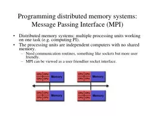
Evolution of Distributed Memory Multiprocessors • Direct queue connections replaced by DMA (direct memory access) • Processor packs or copies messages • Initiates transfer, goes on computing • Message passing libraries provide store-and-forward abstraction • can send/receive between any pair of nodes, not just along one wire • Time proportional to distance since each processor along path must participate • Wormhole routing in hardware • special message processors do not interrupt main processors along path • message sends are pipelined • don’t wait for complete message before forwarding
PRAM • Parallel Random Access Memory • All memory access free • Theoretical, “too good to be true” • OK for understanding whether an algorithm has enough parallelism at all • Slightly more realistic: • Concurrent Read Exclusive Write (CREW) PRAM
Latency and Bandwidth • Time to send message of length n is roughly • Topology irrelevant • Often called “a-b model” and written • Usually a >> b >> time per flop • One long message cheaper than many short ones • Can do hundreds or thousands of flops for cost of one message • Lesson: need large computation to communication ratio to be efficient Time = latency + n*cost_per_word = latency + n/bandwidth Time = a + n*b a + n*b << n*(a + 1*b)
Example communication costs • a and b measured in units of flops, b measured per 8-byte word Machine Year ab Mflop rate per proc CM-5 1992 1900 20 20 IBM SP-1 1993 5000 32 100 Intel Paragon 1994 1500 2.3 50 IBM SP-2 1994 7000 40 200 Cray T3D (PVM) 1994 1974 28 94 UCB NOW 1996 2880 38 180 SGI Power Challenge 1995 3080 39 308 SUN E6000 1996 1980 9 180
P M P M os or L (latency) More detailed performance model: LogP • L: latency across the network • o: overhead (sending and receiving busy time) • g: gap between messages (1/bandwidth) • P: number of processors • People often group overheads into latency (a, b model) • Real costs more complicated • (see Culler/Singh, Chapter 7)
Implementing Message Passing • Many “message passing libraries” available • Chameleon, from ANL • CMMD, from Thinking Machines • Express, commercial • MPL, native library on IBM SP-2 • NX, native library on Intel Paragon • Zipcode, from LLL • … • PVM, Parallel Virtual Machine, public, from ORNL/UTK • MPI, Message Passing Interface, industry standard • Need standards to write portable code • Rest of this discussion independent of which library • Will have detailed MPI lecture later
Implementing Synchronous Message Passing • Send completes after matching receive and source data has been sent • Receive completes after data transfer complete from matching send source destination 1) Initiate send send (Pdest, addr, length,tag) rcv(Psource, addr,length,tag) 2) Address translation on Pdest 3) Send-Ready Request send-rdy-request 4) Remote check for posted receive tag match 5) Reply transaction receive-rdy-reply 6) Bulk data transfer time data-xfer
Example: Permuting Data • Exchanging data between Procs 0 and 1, V.1: What goes wrong? Processor 0 Processor 1 send(1, item0, 1, tag) send(0, item1, 1, tag) recv( 1, item1, 1, tag) recv( 0, item0, 1, tag) • Deadlock • Exchanging data between Proc 0 and 1, V.2: Processor 0 Processor 1 send(1, item0, 1, tag) recv(0, item0, 1, tag) recv( 1, item1, 1, tag) send(0,item1, 1, tag) • What about a general permutation, where Proc j wants to send to • Proc s(j), where s(1),s(2),…,s(P) is a permutation of 1,2,…,P?
Implementing Asynchronous Message Passing • Optimistic single-phase protocol assumes the destination can buffer data on demand source destination 1) Initiate send send (Pdest, addr, length,tag) 2) Address translation on Pdest 3) Send Data Request data-xfer-request tag match allocate 4) Remote check for posted receive 5) Allocate buffer (if check failed) 6) Bulk data transfer rcv(Psource, addr, length,tag) time
Safe Asynchronous Message Passing • Use 3-phase protocol • Buffer on sending side • Variations on send completion • wait until data copied from user to system buffer • don’t wait -- let the user beware of modifying data source destination 1) Initiate send send (Pdest, addr, length,tag) rcv(Psource, addr, length,tag) 2) Address translation on Pdest 3) Send-Ready Request send-rdy-request 4) Remote check for posted receive return and continue tag match record send-rdy computing 5) Reply transaction receive-rdy-reply 6) Bulk data transfer time data-xfer
Example Revisited: Permuting Data • Processor j sends item to Processor s(j), where • s(1),…,s(P) is a permutation of 1,…,P Processor j send_asynch(s(j), item, 1, tag) recv_block( ANY, item, 1, tag) • What could go wrong? • Need to understand semantics of send and receive • Many flavors available
Other operations besides send/receive • “Collective Communication” (more than 2 procs) • Broadcast data from one processor to all others • Barrier • Reductions (sum, product, max, min, boolean and, #, …) • # is any “associative” operation • Scatter/Gather • Parallel prefix • Proc j owns x(j) and computes y(j) = x(1) # x(2) # … # x(j) • Can apply to all other processors, or a user-define subset • Cost = O(log P) using a tree • Status operations • Enquire about/Wait for asynchronous send/receives to complete • How many processors are there • What is my processor number