Download
1 / 59
590 likes | 770 Views
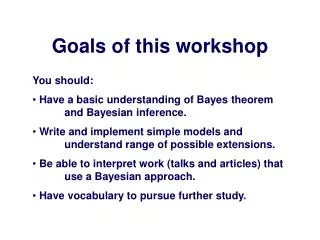
Goals of this workshop. You should: Have a basic understanding of Bayes theorem and Bayesian inference. Write and implement simple models and understand range of possible extensions. Be able to interpret work (talks and articles) that use a Bayesian approach .

E N D
Goals of this workshop • You should: • Have a basic understanding of Bayes theorem and Bayesian inference. • Write and implement simple models and understand range of possible extensions. • Be able to interpret work (talks and articles) that use a Bayesian approach. • Have vocabulary to pursue further study.
Frequentist How likely are these data given model M? Bayesian What is probability of model M given the data?
Frequentist How likely are these data given model M? Data Model Bayesian What is probability of model M given the data? Prior * Data Posterior Model
Do you have TB? …or is it just allergies
Do you have TB? Data: Positive test (+) Is it time to panic?
Do you have TB? Background/Prior Information: Population incidence = 0.01 or 1% Imperfect data: P(+/Inf)= 95% P(-/Inf)= 5% [false negative] P(+/uninf) = 5% [false positive]
Do you have TB? Background/Prior Information: Population incidence = 0.01 or 1% Imperfect data: P(Test +/Inf)= 95% P(-/Inf)= 5% [false negative] P(+/uninf) = 5% [false positive] What is the probability that you have TB, given that you tested positive P(Inf/+) ??
Do you have TB? P(Inf) = 0.01 = Background probability of infection P(+/Inf) = 0.95 P(-/Inf)= 0.05 P(+/uninf) =0.05 The probability that you test + (with or without TB) is sum of all circumstances that might lead to + test, P(+) = P(+/Inf) * P(Inf) + P(+/uninf) * P(uninf) =(0.95*0.01) + (0.05*0.99) = 0.059
What is the probability that you have TB, given that you tested positive? P(Inf/+) = P(+/Inf) * P(Inf) P(+)
What is the probability that you have TB, given that you tested positive? P(Inf/+) = P(+/Inf) * P(Inf) P(+) P(Inf/+) = 0.95* 0.01 = 0.161 0.059 P(Inf) = 0.01 P(+/Inf) = 0.95 P(-/Inf)= 0.05 P(+/uninf) =0.05 P(+) =0.059
What is the probability that you have TB, given that you tested positive? P(Inf/+) = 16% P(Inf) = 0.01 P(+/Inf) = 0.95 P(-/Inf)= 0.05 P(+/uninf) =0.05 P(+) =0.059
What is the probability that you have TB, given that you tested positive? P(Inf/+) = 16% P(Inf) = 0.01 P(+/Inf) = 0.95 P(-/Inf)= 0.05 P(+/uninf) =0.05 P(+) =0.059 1/100 test positive and are positive About 5/100 test positive by accident Of 6 + tests, only 1/6 (16.7%) is actually infected. [Testing + (new data) made you 16% more likely to have TB than you were before the test.]
A Bayesian Analysis uses probability theory (Bayes Theorem) to generate probabilistic inference P(ϴ /y) = P(y/ϴ)P(ϴ) P(y) The posterior distribution (P(ϴ /y) describes the probability model or parameter value ϴ given the data y. P(y/ ϴ ) = likelihood, a base for most statistic paradigms P(ϴ ) = prior, background understanding of model P(y) = marginal likelihood, a normalizing constant to ensure posterior sums to 1.
Some Probability Theory For events A and B, • Pr(A,B) stands for the joint probabilitythat both events happen. • Pr(A|B) is the conditional probability that A happens given that B has occurred. If two events A and B are independent: Pr(A,B) = Pr(A)Pr(B) • Then, • P(A|B) P(B) = P(A,B) • and • P(B|A) P(A) = P(A,B) • It follows that:
What is the probability that you have TB, given that you tested positive? P(Inf/+) = P(+/Inf) * P(Inf) P(+) P(Inf) = 0.50 == An objective (‘noninformative’) prior P(+/Inf) = 0.95 P(-/Inf)= 0.05 P(+/uninf) =0.05 P(+) ==(0.95*0.50) + (0.05*0.99) = 0.50
What is the probability that you have TB, given that you tested positive? P(Inf/+) = P(+/Inf) * P(Inf) P(+) P(Inf) = 0.50 == An objective (‘noninformative’) prior P(+/Inf) = 0.95 P(-/Inf)= 0.05 P(+/uninf) =0.05 P(+) ==(0.95*0.50) + (0.05*0.99) = 0.50 P(Inf/+) = 0.95* 0.05 = 0.95 0.50 *using an uninformative prior just returns the likelihood value, based on an initial belief that 50% people are infected.
The Frequentist definition of probability only applies to inherently repeatable events, e.g., from the vantage point 2013, PF (the Republicans will win the White House again in 2016) is (strictly speaking) undefined. All forms of uncertainty are in principle quantifiable within the Bayesian definition.
Bayesian Model framework Prior * Likelihood (DATA) ~ Posterior Probability P(y/ϴ) P(ϴ)
Bayesian Model framework Prior * Likelihood (DATA) ~ Posterior Probability P(ϴ/y ) P(y/ϴ) P(ϴ)
Bayesian Model framework Prior * Likelihood (DATA) ~ Posterior Probability Mean 95% CI Extremes ... P(ϴ/y )
Data = Y (observations y1…yN) • Parameter =µ • Likelihood for observation y for a normal sampling distribution: y ~ Norm (µ,σ2)
Data = Y (observations y1…yN) • Parameter =µ • Likelihood for observation y for a normal sampling distribution: y ~ Norm (µ,σ2) µ ~ Norm (µ,τ2)
Data = Y • Parameter =µ • Likelihood for observation y for a normal sampling distribution: y ~ Norm (µ,σ2) µ ~ Norm (µ,τ2) P(µ|y, σ, τ) ~ Norm (µ,σ2)
Data = Y (observations y1…yN) • Parameter =µ • Likelihood for dataset Y for a normal sampling distribution: Y ~ Norm (µ,σ2) ]
MCMC Gibbs sampler = Algorithm for I iterations for y~ f(μ,σ): • 1. Select initial values μ(0) and σ(0) • 2. Sample from each conditional posterior distribution, treating the other parameter as fixed. for(1: I){ • sample μ(i)| σ(i-1) • sample σ(i)| μ(i) } This decomposes a complex, multi-dimension problem into a series of one-dimension problems.
Hierarchical Bayes Y = 0 + mX + ɛ ɛ = error (assumed) in data sampling.
Hierarchical Bayes Y = 0 + mX + ɛ ɛ = error (assumed) in data sampling. This error doesn’t get propagated forward in predictions.
Why Hierarchical Bayes? • Ecological systems are complex • Data are a subsample of true population • Increasing demand for accurate forecasts
Why Hierarchical Bayes (HB)? • Ecological systems are complex • Data are a subsample of true population • Increasing demand for accurate forecasts • Analyses should accommodate these realities!
Hierarchical Analysis Hierarchical Model Y ~ mX+b + ɛ Standard Model Z ~x + ɛ.obs Data Process Parameters m, b, ɛ Y ~mZ+b + ɛ.proc m,b, ɛ.proc, ɛ.obs
Hierarchical Analysis Bayesian Hierarchical Model Z ~x + ɛ.obs Data Process Parameters Hyperparameters Y ~mZ+b + ɛ.proc m, b, ɛ.proc, ɛ.obs σ2m, σ2b
Hierarchical Analysis Data: P(Y) ~ Pois(λ) Process: log (λ) = f(state, size, η) η denotes stochasticity, could be random, spatial Parameters: (αp, η) Hyperparameters: (σα, σ η)
Bayesian Hierarchical Analysis The joint distribution [process,parameters| data]= [data|process, parameters] * [process|parameters] * [parameters]
Bayesian Hierarchical Analysis The joint distribution [process,parameters| data]= [data|process, parameters] * [process|parameters] * [parameters] P(P, θ.p, θ.d|D) = (D|P, θ.p, θ.d)*(P, θ.p, θ.d) (D)
Bayesian Hierarchical Analysis The joint distribution [process,parameters| data]= [data|process, parameters] * [process|parameters] * [parameters] Bayes Theorem P(P, θ.p, θ.d|D) = (D|P, θ.p, θ.d)*(P, θ.p, θ.d) (D)
Bayesian Hierarchical Analysis The joint distribution [process,parameters| data]= [data|process, parameters] * [process|parameters] * [parameters] Bayes Theorem P(P, θ.p, θ.d|D) = (D|P, θ.p, θ.d)*(P, θ.p, θ.d) (D) Probability theory shows: ∞(D|P,θ.d)*(P| θ.p)* (θ.p, θ.d) … a series of low dimension conditional distributions.
HB Example Question: Do trees produce more seeds when grown at elevated CO2? Design: 50-100 trees in 6 plots, 3 at ambient and 3 elevated Data: Fecundity time series (#cones) on trees and seeds on ground. [Seeds per pine cone: 83 +/- 24 (no CO2 effect)]
Intervention Trees reach maturity Trees grow Cone counts on FACE trees Data Seed collection at FACE Pretreatment phase Design Fumigation CO2 treatment: reproduction control 1996 1998 2000 2002 2004 The fecundity process is complex… Tree responses 1996 through 1998 ….pretreatment Change of scale: seeds in plots to cones on individuals.
…and nature is tricky. Intervention Mortality Tree responses Trees reach maturity Trees grow Data Cone counts on the FACE trees Seed collection in the FACE Interannual differences Ice storm damage Pretreatment phase Design CO2 treatment fumigation control 1996 1998 2000 2002 2004
Modeling Seed Production • Maturation is estimated for all trees with unknown status. • Fecundity is only modeled for mature trees.
Modeling Seed Production Probability of being mature = f (diameter)
Modeling Seed Production Trees mature at smaller diameters in elevated CO2.More young trees have matured in high CO2.
Seed production = f(CO2, diameter, ice storm, year effects) Modeling Seed Production (# & location) (# & location) Dispersal model and priors: Clark, LaDeau and Ibanez 2004
At diameters of 24 cm to 25 cm mean Ambient cones= 7 mean Elevated cones= 52
Modeling Seed Production Seed production = f(CO2, diameter, ice storm, year effect) Random intercept model: We also allow seed production to vary among individuals.
Mature trees in the high CO2 plots produce up to 125 more cones per tree than mature ambient trees.
* * Wahlenberg 1960 Model predictions suggest even larger enhancement of cone productivity as trees age. Cones per tree (model prediction)