Download
1 / 72
720 likes | 848 Views
Learning to Reason with Extracted Information. William W. Cohen Carnegie Mellon University joint work with: William Wang, Kathryn Rivard Mazaitis , Stephen Muggleton, Tom Mitchell, Ni Lao,

E N D
Learning to Reason with Extracted Information William W. CohenCarnegie Mellon University joint work with: William Wang, Kathryn Rivard Mazaitis, Stephen Muggleton, Tom Mitchell, Ni Lao, Richard Wang, Frank Lin, Ni Lao, Estevam Hruschka, Jr., Burr Settles, Partha Talukdar, Derry Wijaya, Edith Law, Justin Betteridge, Jayant Krishnamurthy, Bryan Kisiel, Andrew Carlson, Weam Abu Zaki , Bhavana Dalvi, Malcolm Greaves, Lise Getoor, Jay Pujara, Hui Miao, …
Motivation • MLNs (and comparable probabilistic first-order logics) are very general tools for constructing learning algorithms • But: they’re computationally expensive • converting to Markov nets: O(nk) • where k is predicate arity, n is the size of the database (#facts about the problem) • inference in Markov nets (even small ones) is intractable • and really should be in the inner loop of the learner
Motivation • What would a tractable version of MLNs look like? • inference would have to be constrained • MLNs allow: (a ^ b c V d) == (~a V ~b V c V d) • Horn clauses: (a ^ b c) == (~a V ~b V c) • but that’s not enough: • even binary (a b) clauses become hard to evaluate as MLNs • you’d have to build a small“network” (or something like it) from a large database • how?
Motivation • What would a tractable version of MLNs look like? • would it still be rich enough to be useful?
Learning about graph similarity:past work • Personalized PageRank aka Random Walk with Restart: basically PageRank where surfer always “teleports” to a start node x. • Query: Given type t* and node x, find y:T(y)=t* and y~x • Answer: ranked list of y’s similar-to x • Einat Minkov’s thesis (2008): Learning parameterized variants of personalized PageRank for PIM and language tasks. • Ni Lao’s thesis (2012): New, better learning methods • richer parameterization: one parameter per “path” • faster inference • Path Ranking Algorithm (PRA)
Lao: A learned random walk strategy is a weighted set of random-walk “experts”, each of which is a walk constrained by a path (i.e., sequence of relations) Recommending papers to cite in a paper being prepared 1) papers co-cited with on-topic papers 6) approx. standard IR retrieval 7,8) papers cited during the past two years 12-13) papers published during the past two years
NELL • Large-scale information extraction system • Learns 100’s of inter-related relations at once • Demo…
These paths are a closely related to logical inference rules(Lao, Cohen, Mitchell 2011)(Lao et al, 2012) Random walk interpretation is crucial Synonyms of the query team i.e. 10-15 extra points in MRR
These paths are a closely related to logical inference rules(Lao, Cohen, Mitchell 2011)(Lao et al, 2012) athletePlaysSport(X,Y) isa(X,Concept), isa(Z,Concept), athletePlaysSport(Z,Y). athletePlaysSport(X,Y) athletePlaysInLeague(X,League), superPartOfOrg(League,Team), teamPlaysSport(Team,Y). Synonyms of the query team path is a continuous feature of a <Source,Destination> pair strength of feature is random-walk probability final prediction is weighted combination of these
A limitation of PRA • Paths are learned separately for each relation type, and one learned rule can’t call another • So, PRA can learn this…. athletePlaySportViaRule(Athlete,Sport) onTeamViaKB(Athlete,Team), teamPlaysSportViaKB(Team,Sport) teamPlaysSportViaRule(Team,Sport) memberOfViaKB(Team,Conference), hasMemberViaKB(Conference,Team2), playsViaKB(Team2,Sport). teamPlaysSportViaRule(Team,Sport) onTeamViaKB(Athlete,Team), athletePlaysSportViaKB(Athlete,Sport)
A limitation • Paths are learned separately for each relation type, and one learned rule can’t call another • But PRA can not learn this….. athletePlaySport(Athlete,Sport) onTeam(Athlete,Team), teamPlaysSport(Team,Sport) athletePlaySport(Athlete,Sport) athletePlaySportViaKB(Athlete,Sport) teamPlaysSport(Team,Sport) memberOf(Team,Conference), hasMember(Conference,Team2), plays(Team2,Sport). teamPlaysSport(Team,Sport) onTeam(Athlete,Team), athletePlaysSport(Athlete,Sport) teamPlaysSport(Team,Sport) teamPlaysSportViaKB(Team,Sport)
So PRA is only single-step inference: known facts inferred facts but not known facts inferred facts more inferred facts … Proposed solution: extend PRA to include large subset of Prolog, a first-order logic athletePlaySport(Athlete,Sport) onTeam(Athlete,Team), teamPlaysSport(Team,Sport) athletePlaySport(Athlete,Sport) athletePlaySportViaKB(Athlete,Sport) teamPlaysSport(Team,Sport) memberOf(Team,Conference), hasMember(Conference,Team2), plays(Team2,Sport). teamPlaysSport(Team,Sport) onTeam(Athlete,Team), athletePlaysSport(Athlete,Sport) teamPlaysSport(Team,Sport) teamPlaysSportViaKB(Team,Sport)
Programming with Personalized PageRank (ProPPR) William Wang Kathryn Rivard Mazaitis
Sample ProPPR program…. features of rules (generated on-the-fly) Horn rules
.. and search space… Insight: This is a graph!
Score for a query soln (e.g., “Z=sport” for “about(a,Z)”) depends on probability of reaching a ☐ node* • learn transition probabilities based on features of the rules • implicit “reset” transitions with (p≥α) back to query node • Looking for answers supported by many short proofs *as in Stochastic Logic Programs [Cussens, 2001] “Grounding” (proof tree) size is O(1/αε) … ie independent of DB size fast approx incremental inference (Reid,Lang,Chung, 08) Learning: supervised variant of personalized PageRank (Backstrom & Leskovic, 2011)
Programming with Personalized PageRank (ProPPR) • Advantages: • Can attach arbitrary features to a clause • Minimal syntactic restrictions: can allow recursion, multiple predicates, function symbols (!), …. • Grounding cost -- conversion to the zero-th order learning problem -- does not depend on the number of known facts in the approximate proof case.
Inference Time: Citation Matchingvs Alchemy “Grounding”cost is independent of DB size
Accuracy: Citation Matching Our rules UW rules AUC scores: 0.0=low, 1.0=hi w=1 is before learning
It gets better….. • Learning uses many example queries • e.g: sameCitation(c120,X) with X=c123+, X=c124-, … • Each query is grounded to a separate small graph (for its proof) • Goal is to tune weights on these edge features to optimize RWR on the query-graphs. • Can do SGD and run RWR separately on each query-graph in parallel • Graphs do share edge features, so there’s some synchronization needed
Learning can be parallelized by splitting on the separate “groundings” of each query
So we can scale: entity-matching problems • Cora bibliography linking: about • 11k facts • 2k train/test queries • TAC KBP entity linking: about • 460,000k facts • 1.2k train/test queries • Timing: • load: 2.5min • train/test: < 1 hour • wall clock time • 8 threads, 20Gb • plausible performance with 8-rule theory
Experiment: • Take top K paths for each predicate learned by PRA • Convert to a mutually recursive ProPPR program • Train weights on entire program athletePlaySport(Athlete,Sport) onTeam(Athlete,Team), teamPlaysSport(Team,Sport) athletePlaySport(Athlete,Sport) athletePlaySportViaKB(Athlete,Sport) teamPlaysSport(Team,Sport) memberOf(Team,Conference), hasMember(Conference,Team2), plays(Team2,Sport). teamPlaysSport(Team,Sport) onTeam(Athlete,Team), athletePlaysSport(Athlete,Sport) teamPlaysSport(Team,Sport) teamPlaysSportViaKB(Team,Sport)
Some details • DB = Subsets of NELL’s KB • Theory = top K PRA rules for each predicate • Test = new facts from later iterations
Some details • DB = Subsets of NELL’s KB • From “ordinary” RWR from seeds: google, beatles, baseball • Vary size by thresholding distance from seeds: M=1k, …, 100k, 1,000k entities then project • Get different “well-connected” subsets • Smaller KB sizes are better-connected easier • Theory = top K PRA rules for each predicate • Test = new facts from later iterations
Some details • DB = Subsets of NELL’s KB • Theory = top K PRA rules for each predicate • For PRA rule p(X,Y) :- q(Y,Z),r(Z,Y) • PRA recursive: q, r can invoke other rules AND p(X,Y) can also be proved via KB lookup via a “base case rule” • PRA non-recursive: q, r must be KB lookup • KB only: only the “base case” rules • Test = new facts from later iterations
Some details • DB = Subsets of NELL’s KB • Theory = top K PRA rules for each predicate • Test = new facts from later iterations • Negative examples from ontology constraints
Results: AUC on test datavarying KB size * KBs overlap a lot at 1M entities
Results: training time in sec inference time as a function of KB size: varying KB from 10k to 50k entities
Outline • Background: information extraction and NELL • Key ideas in NELL • Coupled learning • Multi-view, multi-strategy learning • Inference in NELL • Inference as another learning strategy • Learning in graphs • Path Ranking Algorithm • ProPPR • Structure learning in ProPPR • Conclusions & summary
Structure learning for ProPPR • So far: we’re doing parameter learning on rules learned by PRA and “forced” into a recursive program • Goal: learn structure of rules directly • Learn rules for many relations at once • Every relation can call others recursively • Challenges in prior work: • Inference is expensive! • often approximated, using ~= pseudo-likelihood • Search space for structures is largeanddiscrete until now….
Structure Learning: Example two families and 12 relations: brother, sister, aunt, uncle, …
Structure Learning: Example two families and 12 relations: brother, sister, aunt, uncle, … corresponds to 112 “beliefs”: wife(christopher,penelope), daughter(penelope,victoria), brother(arthur,victoria), … and 104 “queries”: uncle(charlotte,Y) with positive and negative “answers”: [Y=arthur]+, [Y=james]-, … • experiment: • repeat n times • hold out four test queries • for each relation R: • learn rules predicting R from the other relations • test
Structure Learning: Example two families and 12 relations: brother, sister, aunt, uncle, … • Result: • 7/8 tests correct (Hinton 1986) • 78/80 tests correct (Quinlan 1990, FOIL) • but….. • experiment: • repeat n times • hold out four test queries • for each relation R: • learn rules predicting R from the other relations • test
Structure Learning: Example two families and 12 relations: brother, sister, aunt, uncle, … • New experiment (1): • One family is train, one is test • For each relation R: • learn rules defining R in terms of all other relations Q1,…,Qn • Result: 100% accuracy! (with FOIL, c 1990) Alchemy with structure learning is also perfect on 11/12 relations • The Qi’s are background facts / extensional predicates / KB • R for train family are the training queries / intensional preds • R for test family are the test queries
Structure Learning: Example two families and 12 relations: brother, sister, aunt, uncle, … • New experiment (2): • One family is train, one is test • For relation pairs R1,R2 • learn (mutually recursive) rules defining R1 and R2 in terms of all other relations Q1,…,Qn • Result: 0% accuracy! (with FOIL, c 1990) Why? • R1/R2 are pairs: wife/husband, brother/sister, aunt/uncle, niece/nephew, daughter/son
Structure Learning: Example two families and 12 relations: brother, sister, aunt, uncle, … • New experiment (2): • One family is train, one is test • For relation pairs R1,R2 • learn (mutually recursive) rules defining R1 and R2 in terms of all other relations Q1,…,Qn • Result: 0% accuracy! (with FOIL, c 1990) Why? In learning R1, FOIL approximates meaning of R2 using the examples not the partiallylearned program • Typical FOIL result: • uncle(A,B) husband(A,C),aunt(C,B) • aunt(A,B) wife(A,C),uncle(C,B) Alchemy uses pseudo-likelihood, gets 27% MAP on test queries
Structure Learning: Example two families and 12 relations: brother, sister, aunt, uncle, … • New experiment (3): • One family is train, one is test • Use 95% of the beliefs as KB • Use 100% of the training-family beliefs as training • Use 100% of the test-family beliefs as test • Like NELL: learning to complete a KB that has 5% missing data • Result: FOIL MAP is < 65%; Alchemy MAP is < 7.5% • Baseline MAP using incomplete KB: 96.4%
KB Completion New algorithm
Structure learning for ProPPR • Goal: learn structure of rules • Learn rules for many relations at once • Every relation can call others recursively • Challenges in prior work: • Inference is expensive! • often approximated, using ~= pseudo-likelihood • Search space for structures is large and discrete until now…. reduce structure learning to parameter learning via the “Metagol trick” [Muggleton et al]
The “Metagol” Approach • Start with an “abductive second order theory” that defines the space of structures. • Introduce minimal set of assumptions needed to prove that the positive examples are covered. • Each assumption is about the existence of a rule in the learned theory. • Metagol uses iterative deepening to search for minimal assumptions (and hence theory) and learns a “hard” theory. • Here’s how we translate this to ProPPR…
The “Metagol” Approach interp(uncle,joe,Y) interp0(R,Y,joe), abduce_ifInv(uncle,R) kbContains(R,Y,joe), abduce_ifInv(uncle,R) interp(uncle,joe,sam) kbContains(nephew,sam,joe), abduce_ifInv(uncle,nephew) true