Download
1 / 27
270 likes | 464 Views
15.053 Tuesday, March 5 Duality – The art of obtaining bounds – weak and strong duality Handouts: Lecture Notes. Bounds One of the great contributions of optimization theory (and math programming) is the providing of upper

E N D
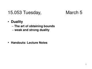
15.053 Tuesday, March 5 • Duality • – The art of obtaining bounds • – weak and strong duality • Handouts: Lecture Notes
Bounds • One of the great contributions of • optimization theory (and math • programming) is the providing of upper • bounds for maximization problems • We can prove that solutions are optimal • For other problems, we can bound the • distance from optimality
A 4-variable linear program • David has minerals that he will mix together and sell • for profit. The minerals all contain some gold • content, and he wants to ensure that the mixture has • 3% gold, and each bag will weigh 1 kilogram. • Mineral 1: 2% gold, $3 profit/kilo • Mineral 2: 3% gold, $4 profit/kilo • Mineral 3: 4% gold, $6 profit/kilo • Mineral 4: 5% gold, $8 profit/kilo maximize z = 3x1 + 4x2 +6x3 + 8x4 subject to x1+ x2 + x3 + x4 = 1 2x1+ 3x2+4x3+ 5x4 = 3 x1, x2, x3, x4≥ 0
A 4-variable linear program maximize z = 3x1 + 4x2 +6x3 + 8x4 subject to x1+ x2 + x3 + x4 = 1 2x1+ 3x2+4x3+ 5x4 = 3 x1, x2, x3, x4≥ 0
Obtaining a Bound Subtract 8 times constraint 1 from the objective function. -z – 5 x1 – 4 x2 – 2 x3 = -8 z + 5 x1 + 4x2 + 2 x3 = 8 Does this show that z ≤ 8? YES!
Obtaining a Second Bound: Treat the operation as pricing out Prices Subtract 3 * constraint 1 and subtract constraint 2 from the objective function. -z – 2x1 – 2 x2 – 1x3 = -6 z + 2 x1 + 2x2 + 1 x3 = 6 Thus z ≤ 6! Which bound is better: 6 or 8?
Obtaining the Best Bound: Formulate the problem as an LP Prices A: 3 - y1- 2y2≤ 0 y1 + 2y2≥ 3 minimize y1 + 3y2 B: 4 - y1- 3y2≤ 0 y1 + 3y2≥ 4 C: 6 - y1- 4y2≤ 0 y1 + 4y2≥ 6 D: 8 - y1- 5y2≤ 0 y1 + 5y2≥ 8
The problem that we formed is called the dual problem minimize y1+ 3y2 Subject to y1+ 2y2 ≥3 y1+ 3y2 ≥4 y1+ 4y2 ≥ 6 y1+ 5y2 ≥ 8 y1 a nd y2 are unconstrained in sign
Summary of previous slides • If “reduced costs” are non-positive then we have • an upper bound on the objective value • The problem of finding the least upper bound is a • linear program, and is referred to as the dual of • the original linear program. • To do: express duality in general notation. • To do: show that the shadow prices solve the • dual, and the bound is the optimal solution to the • original problem
PRIMAL PROBLEM: maximize z = 3x1 + 4x2 +6x3 + 8x4 x1 + x2 + x3 + x4 = 1 2x1 + 3x2 +4x3 + 5x4 = 3 x1, x2, x3, x4≥ 0 subject to Observation 1. The constraint matrix in the primal is the transpose of the constraint matrix in the dual. DUSL PROBLEM: maximize y1+ 3y2 subject to y1+ 2y2 ≥3 Observation 2. The RHS coefficients in the primal become the cost coefficients in the dual. y1+ 3y2 ≥ 4 y1+ 4y2 ≥ 6 y1+ 5y2 ≥ 8
PRIMAL PROBLEM: maximize z = 3x1 + 4x2 +6x3 + 8x4 x1 + x2 + x3 + x4 = 1 2x1 + 3x2 +4x3 + 5x4 = 3 x1, x2, x3, x4≥ 0 subject to Observation 3. The cost coefficients in the primal become the RHS coefficients in the dual. DUSL PROBLEM: Observation 4. The primal (in this case) is a max problem with equality constraints and non-negative variables maximize y1+ 3y2 subject to y1+ 2y2 ≥3 y1+ 3y2 ≥ 4 The dual (in this case) is a minimization problem with ≥ constraints and variables unconstrained in sign. y1+ 4y2 ≥ 6 y1+ 5y2 ≥ 8
PRIMAL PROBLEM (in standard form): max z = c1x1 + c2x2 + c3x3 + … + cnxn s.t. a11x1 + a12x2 + a13x3 + … + a1nxn = b1 a21x1 + a22x2 + a23x3 + … + a2nxn = b2 … am1x1 + am2x2 + am3x3 + … + amnxn = bm xj≥ 0 for j = 1 to n. DUAL PROBLEM: max v = ??? s.t. ??? What is the dual problem in terms of the notation given above?
PRIMAL PROBLEM (in standard form): max z = c1x1 + c2x2 + c3x3 + … + cnxn s.t. a11x1 + a12x2 + a13x3 + … + a1nxn = b1 a21x1 + a22x2 + a23x3 + … + a2nxn = b2 … am1x1 + am2x2 + am3x3 + … + amnxn = bm xj≥ 0 for j = 1 to n. DUAL PROBLEM: max v = b1y1 + b2y2 + b3y3 + … +bnyn s.t. a11y1 + a21y2 + a31y3 + … + am1ym≥ c1 a12y1 + a22y2 + a32y3 + … + am2ym≥ c2 … a1ny1 + a2ny2 + a3ny3 + … + amnym ≥ cn
Weak Duality Theorem Theorem. Suppose that x is any feasible solution to the primal, andy is any feasible solution to the dual. Then Σj=1..n cjxj ≤ Σ i=1..nyi bi(Max ≤ Min) Proof. Σj=1..n cjxj ≤ Σ i=1...nΣ j=1...m (yi aij )xi ≤ Σj=1...mΣi=1...nyi (aijxj) ≤ Σj=1...myi bi
Unboundedness Property Theorem. Suppose that the primal (dual) problem has an unbounded solution. Then the dual (primal) problem has no feasible solution. Proof. Suppose thaty was feasible for the dual. Then every solution to the primal problem is unbounded above by Σj=1...myi bi
Strong Duality Theorem Theorem. If the primal problem has a finite optimal solution value, then so does the dual problem, and these two values are the same.
Strong Duality Illustrated Prices Optimal dual solution: y1 = –1/3, y2 = 5/3, v = 14/3 Optimal primal solution: x1 = 2/3, x2 = 0, x3 = 0, x4 = 1/3 z = 14/3
Strong Duality Illustrated: the final tableau Observation The cost coeffients satisfy complementary slackness Optimal primal solution: x1 = 2/3, x2 = 0, x3 = 0, x4 = 1/3 v = 14/3
Summary • If we take an LP in standard form (max), • we can formulate a dual problem • • Weak Duality: Each solution of the dual • gives an upper bound on the maximum • objective value for the primal • Strong duality: if there are feasible • solutions to the primal and dual, then the • optimal objective value for both problems • is the same.
Shadow prices solve the dual! • Theorem. Suppose that the primal problem • has a finite optimal solution value. Then the • shadow prices for the primal problem form an • optimal solution to the dual problem. (And the • objective values are the same.) David’s Mineral Problem
Shadow prices FACT: Optimal simplex multipliers are shadow prices.
Summary • The dual problem to a maximizing LP • provides upper bounds on the optimal • objective function • The maximum solution value for the • primal is the same as the minimum • solution value for the dual • The shadow prices are optimal for the dual • LP • Next: alternative optimality conditions
Primal Problem max Σj=1..m cj xj s.t. Σj=1..n aij xj = bi for i = 1 to m xj ≥ 0 for all j = 1 to n Optimality Condition 1. A solution x* is optimal for the primal problem if it is a basic feasible solution and the tableau satisfies the optimality conditions. Optimality Condition 2. A solution x* is optimal for the primal problem if it is feasible and if there is a feasible solution y* for the dual with Σj=1..m cj x*j = Σj=1..m y*i bi Dual Problem min Σj=1..m yi bi s.t. Σi=1..m yi aij ≥ cj for j = 1 to n
Complementary Slackness Conditions. – Suppose thaty is feasible for the dual, and let cj= cj - Σi=1..myi aij . Supposex is feasible for the primal. Theorem(complementary slackness). x andy are optimal for the primal and dual if and only if cjxj = 0 for all j. Primal Problem max Σj=1..m cj xj s.t. Σj=1..n aij xj = bi for i = 1 to m xj ≥ 0 for all j = 1 to n Dual Problem min Σj=1..m yi bi s.t. Σi=1..m yi aij ≥ cj for j = 1 to n
Next Lecture on Duality • Dual linear programs in general form • Optimality Conditions in general form. • Illustrating Duality with 2-person 0-sum • game theory
Coverage for first midterm (Closed book exam) • Formulations • 2D graphing and • finding opt. solution • Setting up an LP in • standard form • The simplex algorithm • starting with a bfs • Phase 1 of the • simplex algorithm • Interpreting sensitivity • analysis, including • shadow prices, and • ranges, and reduced • costs • Pricing out • Using tableaus to • determine shadow • prices, reduced costs, • and ranges