Ch. 12: Perfect Competition.
270 likes | 447 Views
Ch. 12: Perfect Competition. Selection of price and output Shut down decision in short run. Entry and exit behavior. Predicting the effects of a change in demand, technological advance, or change in cost. Efficiency of perfect competition. Perfect Competition.

Ch. 12: Perfect Competition.
E N D
Presentation Transcript
Ch. 12: Perfect Competition. • Selection of price and output • Shut down decision in short run. • Entry and exit behavior. • Predicting the effects of a change in demand, technological advance, or change in cost. • Efficiency of perfect competition
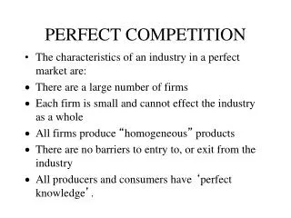
Perfect Competition • Perfect competition is an industry in which: • Many firms sell identical products to many buyers. • No barriers to entry. • Established firms have no advantages over new ones. • Sellers and buyers are well informed about prices. • Perfect competition arises when • When firm’s minimum efficient scale is small relative to market demand • Homogeneous products – only price matters to buyers.
Perfect Competition • In perfect competition, each firm is a price taker. • No single firm can influence the price • Each firm’s output is a perfect substitute for the output of the other firms, • Demand for each firm’s output is perfectly elastic.
Perfect Competition • Market demand and supply determine the price that the firm must take. • A firm’s marginal revenue is the change in TR resulting from a one-unit increase in the quantity sold. • In perfect competition, MR=P.
Perfect Competition • Firms’s goal: maximize economic profit. • = TR – TC TR=PXQ TC=opportunity costs of production, including normal profit for the owner.
Profit Max. in Perfect Comp. A perfectly competitive firm faces two constraints: • A market constraint summarized by the market price and the firm’s revenue curves • A technology constraint summarized by firm’s product curves and cost curves.
Profit Max. in Perfect Comp. • 2 decisions in the short run: • Whether to produce or to shut down. • If the decision is to produce, what quantity to produce. • A firm’s long-run decisions are: • Whether to stay in the industry or leave it. • Whether to increase or decrease its plant size.
Profit Max. in Perfect Comp. • At low output levels, the firm incurs an economic loss—it can’t cover its fixed costs. • Profits maximized at 9 units of output.
Profit Max. in Perfect Comp. • Marginal Analysis • Because MR is constant and MC eventually increases as output increases, profit is maximized by producing the output at which (P=)MR = MC
Profit Max. in Perfect Comp. • Profit = (P-ATC)*Q
Profit Max. in Perfect Comp. • SR decision to shut down. • P = (P-ATC)*Q • = (P-AVC)*Q –TFC • If P < minimum of AVC, the firm shuts down temporarily and incurs a loss equal to TFC. • If P> minimum of AVC, the firm produces the quantity at which P=MC, even if profits are negative.
Profit Max. in Perfect Comp. • The Firm’s Short-Run Supply Curve • shows how the firm’s profit-maximizing output varies as the market price varies, other things remaining the same. • MC curve above minimum of AVC
Graphic representation of firm’s profit maximizing output for various prices
SR Industry Supply Curve • The quantity supplied by the industry at any given price is the sum of the quantities supplied by all the firms in the industry at that price. • Entry of new firms shifts industry supply curve to the right • Exit of old firms shifts industry supply curve to the left.
LR adjustments • In SR, economic profits could be positive, negative or zero. • In the LR, • Firms enter if economic profits are positive • Firms exit if economic profits are negative. • No entry or exit if economic profits are zero.
LR adjustments • Effect of increase in demand on economic profits in LR • At LR equilibrium • P=MC=ATC • P=0 • ATC is at a minimum
SR vs. LR Adjustments • Summary of effects of an increase in demand when starting from a LR equilibrium.
LR equilibrium Long-run equilibrium occurs in a competitive industry when: • P is zero, so firms have no incentive to enter or exit the industry. • LRATC is at its minimum, so firms can’t reduce costs by changing plant size.
External Economies and Diseconomies • Constant cost industry • Industry output has no effect on a given firm’s ATC • External economies • decreasing cost industry • Firm’s costs fall as industry output rises • External diseconomies • Increasing cost industry • Firm’s costs rise as industry output rises
External Economics and Diseconomies • LR supply curve reflects how change in industry output affects ATC. • External economies LR supply upward sloping • External diseconomies LR supply downward sloping • Constant cost industry LR supply horizontal.
LR adjustment to change in demand with decreasing cost industry
LR adjustment to change in demand with increasing cost industry
Changes in Plant Size or adoption of new technology • Firms change their production technology (or plant size) whenever doing so is profitable. • If ATC exceeds the minimum of LRATC, firms change their technology to lower costs and increase profits. • Suppose a new technology emerges that reduces LRATC at a higher level than previously.
Changes in Production Technology • Why can’t a firm survive in LR at Q=6? • Why is LR equilibrium at Q where LRATC is minimized?
Technological Advances • New-technology firms enter and old-technology firms either exit or adopt the new technology. • Optimal sized firm could be either larger or smaller • Industry supply increases and the industry supply curve shifts rightward. • The price falls and the quantity increases. • Eventually, a new long-run equilibrium emerges in which • all the firms use the new technology • the price has fallen to the minimum average total cost • each firm earns normal profit (zero economic profit)
Competition and Efficiency • Competitive equilibrium is efficient only if there are no external benefits or costs. • Positive externalities. • Negative externalities.