Download
1 / 24
250 likes | 317 Views
Learn about Continuous and Discrete Fourier Series, Fast Fourier Transform, applications in industry, medical, speech analysis, and a brief history of Fourier analysis development.

E N D
Lecture on Fourier Analysis www.AssignmentPoint.com www.assignmentpoint.com
TOPICS 1. Frequency analysis: a powerful tool 2. A tour of Fourier Transforms 3. Continuous Fourier Series (FS) 4. Discrete Fourier Series (DFS) 5. Example: DFS by DDCs & DSP www.assignmentpoint.com
analysis General Transform as problem-solving tool s(t), S(f) : Transform Pair time, tfrequency, f F s(t) S(f) = F[s(t)] synthesis Frequency analysis: why? • Fast & efficient insight on signal’s building blocks. • Simplifies original problem - ex.: solving Part. Diff. Eqns. (PDE). • Powerful & complementary to time domain analysis techniques. • Several transforms in DSPing: Fourier, Laplace, z, etc. www.assignmentpoint.com
Fourier analysis - applications • Applications wide ranging and ever present in modern life • Telecomms - GSM/cellular phones, • Electronics/IT - most DSP-based applications, • Entertainment - music, audio, multimedia, • Accelerator control (tune measurement for beam steering/control), • Imaging, image processing, • Industry/research - X-ray spectrometry, chemical analysis (FT spectrometry), PDE solution, radar design, • Medical - (PET scanner, CAT scans & MRI interpretation for sleep disorder & heart malfunction diagnosis, • Speech analysis (voice activated “devices”, biometry, …). www.assignmentpoint.com
Periodic (period T) FS Discrete Continuous Aperiodic FT Continuous ** Periodic (period T) DFS Discrete Discrete DTFT Continuous Aperiodic ** DFT Discrete ** Calculated via FFT Note: j =-1, = 2/T, s[n]=s(tn), N = No. of samples Fourier analysis - tools Input Time Signal Frequency spectrum www.assignmentpoint.com
A little history • Astronomic predictions by Babylonians/Egyptians likely via trigonometric sums. • 1669: Newton stumbles upon light spectra (specter = ghost) but fails to recognise “frequency” concept (corpuscular theory of light, & no waves). • 18th century: two outstanding problems • celestial bodies orbits: Lagrange, Euler & Clairaut approximate observation data with linear combination of periodic functions; Clairaut,1754(!) first DFT formula. • vibrating strings: Euler describes vibrating string motion by sinusoids (wave equation). BUT peers’ consensus is that sum of sinusoids only represents smooth curves. Big blow to utility of such sums for all but Fourier ... • 1807: Fourier presents his work on heat conduction Fourier analysis born. • Diffusion equation series (infinite) of sines & cosines. Strong criticism by peers blocks publication. Work published, 1822 (“Theorie Analytique de la chaleur”). www.assignmentpoint.com
A little history -2 • 19th / 20th century: two paths for Fourier analysis - Continuous & Discrete. CONTINUOUS • Fourier extends the analysis to arbitrary function (Fourier Transform). • Dirichlet, Poisson, Riemann, Lebesgue address FS convergence. • Other FT variants born from varied needs (ex.: Short Time FT - speech analysis). DISCRETE: Fast calculation methods (FFT) • 1805 - Gauss, first usage of FFT (manuscript in Latin went unnoticed!!! Published 1866). • 1965 - IBM’s Cooley & Tukey “rediscover” FFT algorithm (“An algorithm for the machine calculation of complex Fourier series”). • Other DFT variants for different applications (ex.: Warped DFT - filter design & signal compression). • FFT algorithm refined & modified for most computer platforms. www.assignmentpoint.com
A periodic function s(t) satisfying Dirichlet’s conditions * can be expressed as a Fourier series, with harmonically related sine/cosine terms. a0, ak, bk : Fourier coefficients. k: harmonic number, T: period, = 2/T For all t but discontinuities (signal average over a period, i.e. DC term & zero-frequency component.) * see next slide Fourier Series (FS) synthesis analysis Note: {cos(kωt), sin(kωt) }k form orthogonal base of function space. www.assignmentpoint.com
Dirichlet conditions (a) s(t) piecewise-continuous; s(t) piecewise-monotonic; s(t) absolutely integrable , (b) In any period: (c) Rate of convergence Example: square wave if s(t) discontinuous then |ak|<M/k for large k (M>0) (a) (b) (c) FS convergence www.assignmentpoint.com
FS of odd* function: square wave. (zero average) (odd function) *Even & Odd functions Even : s(-x) = s(x) Odd : s(-x) = -s(x) FS analysis - 1 www.assignmentpoint.com
Fourier spectrum representations Rectangular Polar vk = akcos(k t) - bksin(k t) vk =rk cos (k t + k) rK = amplitude, K= phase fk=k /2 Fourier spectrum of square-wave. FS analysis - 2 www.assignmentpoint.com
FS synthesis Square wave reconstruction from spectral terms Convergence may be slow (~1/k) - ideally need infinite terms. Practically, series truncated when remainder below computer tolerance ( error). BUT … Gibbs’ Phenomenon. www.assignmentpoint.com
First observed by Michelson, 1898. Explained by Gibbs. • Max overshoot pk-to-pk = 8.95% of discontinuity magnitude. • Just a minor annoyance. • FS converges to (-1+1)/2 = 0 @ discontinuities, in this case. Gibbs phenomenon Overshoot exist @ each discontinuity www.assignmentpoint.com
(zero average) amplitude (even function) phase FS time shifting FS of even function: /2-advanced square-wave Note: amplitudes unchanged BUTphases advance by k/2. www.assignmentpoint.com
Euler’s notation: e-jt = (ejt)* = cos(t) - j·sin(t) “phasor” Complex form of FS (Laplace 1782). Harmonics ck separated by f = 1/T on frequency plot. Link to FS real coeffs. Complex FS analysis synthesis Note: c-k = (ck)* www.assignmentpoint.com
Homogeneity a·s(t) a·S(k) Additivity s(t) + u(t) S(k)+U(k) Linearity a·s(t) + b·u(t) a·S(k)+b·U(k) Time reversal s(-t) S(-k) Multiplication* s(t)·u(t) Convolution* S(k)·U(k) Time shifting Frequency shifting S(k - m) *Explained in next week’s lecture FS properties Time Frequency www.assignmentpoint.com
Orthonormal base Fourier components {uk} form orthonormal base of signal space: uk = (1/T) exp(jkωt) (|k| = 0,1 2, …+) Def.: Internal product : uk um = δk,m (1 if k = m, 0 otherwise). (Remember (ejt)* = e-jt ) Then ck = (1/T) s(t) uk i.e. (1/T) times projection of signal s(t) on component uk Negative frequencies & time reversal k = - , … -2,-1,0,1,2, …+ , ωk = kω, k = ωkt, phasor turns anti-clockwise. Negative k phasor turns clockwise (negative phase k ),equivalent to negative time t, time reversal. Careful: phases important when combining several signals! FS - “oddities” www.assignmentpoint.com
Average power W : Parseval’s Theorem Example Pulse train, duty cycle = 2 t / T Wk = 2 W0sync2(k ) bk = 0 a0 = sMAX W0 = ( sMAX)2 sync(u) = sin( u)/( u) ak = 2sMAXsync(k ) FS - power • FS convergence ~1/k • lower frequency terms • Wk = |ck|2 carry most power. • Wk vs. ωk: Power density spectrum. www.assignmentpoint.com
FS of main waveforms www.assignmentpoint.com
Band-limited signal s[n], period = N. DFS defined as: Orthogonality in DFS: ~ ~ Note: ck+N = ck same period N i.e. time periodicity propagates to frequencies! Kronecker’s delta Synthesis: finite sum band-limited s[n] Discrete Fourier Series (DFS) DFS generate periodic ck with same signal period analysis synthesis N consecutive samples of s[n] completely describe s in time or frequency domains. www.assignmentpoint.com
s[n]: period N, duty factor L/N amplitude phase DFS analysis DFS of periodic discrete 1-Volt square-wave Discrete signals periodic frequency spectra. Compare to continuous rectangular function (slide # 10, “FS analysis - 1”) www.assignmentpoint.com
Homogeneitya·s[n] a·S(k) Additivity s[n] + u[n] S(k)+U(k) Linearity a·s[n] + b·u[n] a·S(k)+b·U(k) Multiplication* s[n] ·u[n] Convolution* S(k)·U(k) Time shifting s[n - m] Frequency shifting S(k - h) * Explained in next week’s lecture DFS properties Time Frequency www.assignmentpoint.com
(1) (2) (3) (2) (1) tn = n/fS , n = 1, 2 .. NS, NS= No. samples I[tn ]+j Q[tn ] = s[tn ] e -jLOtn (3) I[tp ]+j Q[tp ] p = 1, 2 .. NT , Ns / NT= decimation. (Down-converted to baseband). DFS analysis: DDC + ... s(t) periodic with period TREV (ex: particle bunch in “racetrack” accelerator) www.assignmentpoint.com
Example: Real-life DDC Fourier coefficients a k*, b k* harmonic k* = LO/REV ... + DSP DDCs with different fLO yield more DFS components www.assignmentpoint.com