Download
1 / 58
1.11k likes | 2.23k Views
Antennas. Theory, characteristics, and implementations. Topics. Role of antennas Theory Antenna types Characteristics Radiation pattern – beamwidth, pattern solid angle Directivity, gain, effective area Bandwidth Friis’ transmission formula Implementations

E N D
Antennas Theory, characteristics, and implementations
Topics Role of antennas Theory Antenna types Characteristics • Radiation pattern – beamwidth, pattern solid angle • Directivity, gain, effective area • Bandwidth Friis’ transmission formula Implementations • Dipole, monopole, and ground planes • Horn • Parabolic reflector • Arrays Terminology
The role of antennas Antennas serve four primary functions • Spatial filter directionally-dependent sensitivity • Polarization filter polarization-dependent sensitivity • Impedance transformer transition between free space and transmission line • Propagation mode adapter from free-space fields to guided waves (e.g., transmission line, waveguide)
Spatial filter Antennas have the property of being more sensitive in one direction than in another which provides the ability to spatially filter signals from its environment. Radiation pattern of directive antenna. Directive antenna.
Polarization filter Antennas have the property of being more sensitive to one polarization than another which provides the ability to filter signals based on its polarization. In this example, h is the antenna’s effective height whose units are expressed in meters.
Impedance transformer Intrinsic impedance of free-space, E/H Characteristic impedance of transmission line, V/I A typical value for Z0 is 50 . Clearly there is an impedance mismatch that must be addressed by the antenna.
Propagation mode adapter In free space the waves spherically expand following Huygens principle:each point of an advancingwave front is in fact thecenter of a fresh disturbanceand the source of a new train of waves. Within the sensor, the waves are guided within a transmission line or waveguide that restricts propagation to one axis.
Propagation mode adapter During both transmission and receive operations the antenna must provide the transition between these two propagation modes.
Antenna types Antennas come in a wide variety of sizes and shapes Helical antenna Horn antenna Parabolic reflector antenna
Theory Antennas include wire and aperture types. Wire types include dipoles, monopoles, loops, rods, stubs, helicies, Yagi-Udas, spirals. Aperture types include horns, reflectors, parabolic, lenses.
Theory In wire-type antennas the radiation characteristics are determined by the current distribution which produces the local magnetic field. Yagi-Uda antenna Helical antenna
Theory – wire antenna example Some simplifying approximations can be made to take advantage the far-field conditions.
Theory – wire antenna example Once Eq and Ef are known, the radiation characteristics can be determined. Defining the directional function f (q, f) from
Theory – aperture antennas In aperture-type antennas the radiation characteristics are determined by the field distribution across the aperture. Horn antenna Parabolic reflector antenna
Theory – aperture antenna example The far-field radiation pattern can be found from the Fourier transform of the near-field pattern. Where Sr is the radial component of the power density, S0 is the maximum value of Sr, and Fn is the normalized version of the radiation pattern F(q, f)
Theory Reciprocity If an emf is applied to the terminals of antenna A and the current measured at the terminals of another antenna B, then an equal current (both in amplitude and phase) will be obtained at the terminals of antenna A if the same emf is applied to the terminals of antenna B. emf: electromotive force, i.e., voltage Result – the radiation pattern of an antenna is the same regardless of whether it is used to transmit or receive a signal.
Characteristics Radiation pattern Radiation pattern – variation of the field intensity of an antenna as an angular function with respect to the axis Three-dimensional representation of the radiation pattern of a dipole antenna
Characteristics Radiation pattern Spherical coordinate system
Characteristics Beamwidth and beam solid angle The beam or pattern solid angle, p [steradians or sr] is defined as where d is the elemental solid angle given by
Characteristics Directivity, gain, effective area Directivity – the ratio of the radiation intensity in a given direction from the antenna to the radiation intensity averaged over all directions. [unitless] Maximum directivity, Do, found in the direction (, ) where Fn= 1 and or Given Do, D can be found
Characteristics Directivity, gain, effective area Gain – ratio of the power at the input of a loss-free isotropic antenna to the power supplied to the input of the given antenna to produce, in a given direction, the same field strength at the same distance Of the total power Pt supplied to the antenna, a part Po is radiated out into space and the remainder Pl is dissipated as heat in the antenna structure. The radiation efficiencyhl is defined as the ratio of PotoPt Therefore gain, G, is related to directivity, D, as And maximum gain, Go, is related to maximum directivity, Do, as
Characteristics Directivity, gain, effective area Effective area – the functional equivalent area from which an antenna directed toward the source of the received signal gathers or absorbs the energy of an incident electromagnetic wave It can be shown that the maximum directivity Do of an antenna is related to an effective area (or effective aperture) Aeff, by where Ap is the physical aperture of the antenna and ha = Aeff / Ap is the aperture efficiency (0 ≤ ha ≤ 1) Consequently [m2] For a rectangular aperture with dimensions lxandly in the x- and y-axes, and an aperture efficiency ha = 1, we get [rad] [rad]
Characteristics Directivity, gain, effective area Therefore the maximum gain and the effective area can be used interchangeably by assuming a value for the radiation efficiency (e.g., l = 1) Example: For a 30-cm x 10-cm aperture, f = 10 GHz ( = 3 cm)xz 0.1 radian or 5.7°, yz 0.3 radian or 17.2°G0 419 or 26 dBi (dBi: dB relative to an isotropic radiator)
Characteristics Bandwidth The antenna’s bandwidth is the range of operating frequencies over which the antenna meets the operational requirements, including: • Spatial properties (radiation characteristics) • Polarization properties • Impedance properties • Propagation mode properties Most antenna technologies can support operation over a frequency range that is 5 to 10% of the central frequency (e.g., 100 MHz bandwidth at 2 GHz) To achieve wideband operation requires specialized antenna technologies (e.g., Vivaldi, bowtie, spiral)
Friis’ transmission formula At a fixed distance R from the transmitting antenna, the power intercepted by the receiving antenna with effective aperture Ar is where Sr is the received power density (W/m2), and Gt is the peak gain of the transmitting antenna.
Friis’ transmission formula If the radiation efficiency of the receiving antenna is hr, then the power received at the receiving antenna’s output terminals is Therefore we can write which is known as Friis’ transmission formula
Friis’ transmission formula as Friis’ transmission formula can be rewritten to explicitly represent the free-space transmission loss, LFS which represents the propagation loss experienced in transmission between two lossless isotropic antennas.With this definition, the Friis formula becomes
Friis’ transmission formula Finally, a general form of the Friis’ transmission formula can be written that does not assume the antennas are oriented to achieve maximum power transfer where (t, t) is the direction of the receiving antenna in the transmitting antenna coordinates, and vice versa for (r, r). An additional term could be included to represent a polarization mismatch between the transmit and receive antennas.
Implementation Dipole, monopole, and ground planes Horns Parabolic reflectors Arrays
ImplementationDipole, monopole, and ground plane For a center-fed, half-wave dipole oriented parallel to the z axis (V/m) (W/m2) Tuned half-wave dipole antenna
Dipole antennas Versions of broadband dipole antennas
Monopole antenna q q Ground plane Radition pattern of vertical monopole above ground of (A) perfect and (B) average conductivity Mirroring principle creates image of monopole, transforming it into a dipole
Ground plane A ground plane will produce an image of nearby currents. The image will have a phase shift of 180° with respect to the original current. Therefore as the current element is placed close to the surface, the induced image current will effectively cancel the radiating fields from the current. The ground plane may be any conducting surface including a metal sheet, a water surface, or the ground (soil, pavement, rock). Horizontal current element Conducting surface(ground plane) Current element image
Implementation Parabolic reflector antennas Circular aperture with uniform illumination. Aperture radius = a. Ap = p a2 where where J1( ) is the Bessel function of the first kind, zero order
Implementation Antenna arrays Antenna array composed of several similar radiating elements (e.g., dipoles or horns). Element spacing and the relative amplitudes and phases of the element excitation determine the array’s radiative properties. Linear array examples Two-dimensional array of microstrip patch antennas
Implementation Antenna arrays The far-field radiation characteristics Sr(, ) of an N-element array composed of identical radiating elements can be expressed as a product of two functions: Where Fa(, ) is the array factor, and Se(, ) is the power directional pattern of an individual element. This relationship is known as the pattern multiplication principle. The array factor, Fa(, ), is a range-dependent function and is therefore determined by the array’s geometry. The elemental pattern, Se(, ), depends on the range-independent far-field radiation pattern of the individual element. (Element-to-element coupling is ignored here.)
Implementation Antenna arrays In the array factor, Ai is the feeding coefficient representing the complex excitation of each individual element in terms of the amplitude, ai, and the phase factor, i, as and ri is the range to the distant observation point.
Implementation Antenna arrays For a linear array with equal spacing d between adjacent elements, which approximates to For this case, the array factor becomes Note that the e-jkR term which is common to all of the summation terms can be neglected as it evaluates to 1.
Implementation Antenna arrays By adjusting the amplitude and phase of each elements excitation, the beam characteristics can be modified.