Download
1 / 42
420 likes | 533 Views
Theoretical Results on Base Station Movement Problem for Sensor Network. Yi Shi ( 石毅 ) and Y. Thomas Hou ( 侯一釗 ) Virginia Tech, Dept. of ECE. IEEE Infocom 2008. Outline. Introduction Problem Constrained Mobile Base Station (C-MB) Problem

E N D
Theoretical Results on Base Station Movement Problem for Sensor Network Yi Shi (石毅) and Y. Thomas Hou (侯一釗 ) Virginia Tech, Dept. of ECE IEEE Infocom 2008
Outline • Introduction • Problem • Constrained Mobile Base Station (C-MB) Problem • Unconstrained Mobile Base Station (U-MB) Problem • Approach • C-MB Problem • Optimal Solution • U-MB Problem • (1-)-approximate solution • Numerical Results • Conclusion
Introduction BS • Sensor Networks • Sensors: gather data, transmit and relay data packets • Low computation power • Battery power • Small storage space • Base station: data collector • Network Lifetime • The first time instance when any of the sensors runs out of energy. • The first time instance when half of the sensors runs out of energy. • The first time instance when the network connectivity is broken up. VCLAB ezLMS references: [1] [2]
Problem • Network Model • The BS is movable • Each sensor node i generates data at rate ri • Data is transmitted to base station via multi-hop • Initial energy at sensor node i is ei • Energy Consumption Modeling • Transmission power modeling where • Receiving power modeling fij: data rate i j dij: distance fki: data rate i
Goal: Find an optimal moving path for the base station such that the network lifetime is maximized. Optimize base station location (x, y)(t) at any time tsuch that the network lifetime is maximized. outgoing data rate incoming data rate gki gij ri Network lifetime i flow balance: Energy constraint The position of the BS Time-dependent Unconstrained Mobile Base Station Problem (U-MB) Problem Formulation
Constrained Mobile Base Station Problem (U-MB) • The base station is only allowed to be present at a finite set of pre-defined points. • For example: (x, y)(t) p1, p2, p3, p4, p5 } Goal: p1 Find an optimal time-dependent location sequences such that the network lifetime is maximized. p3 p5 p2 p4 Time-dependent location sequences: t1 p1 t3 p3 t4 p2 t p1 t2 p4 ……
The Roadmap of the Theoretical Analysis t1 p1 t3 p3 t4 p2 t2 p4 …… • C-MB Problem • Transform the problem from time domain to space domain • Theorem 1 • Linear programming • Optimal Solution • U-MB Problem • Change infinite search space to finite search points • U-MB C-MB • (1-)-approximate solution by solving C-MB on the finite search points • Theorem 2 and 3 p1 t1 p3 t3 p4 t4 p2 t2 ……
C-MB ProblemFrom time-domain to space-domain [0, 50] p1 [50, 90] p2 [90, 100] p2 [100, 130] p1 • Time Domain:
C-MB ProblemFrom time-domain to space-domain p1 [0, 50] + [100, 130] p2 [50, 100] • Space domain:
From Time Domain to Space Domain (cont’d) • Data routing only depends on base station location; not time Theorem
Linear programming Formulation W(p): the cumulative time periods for the BS to be present at location p. Location-dependent fki(p): normalized data rate
A (1 − ε) Optimal Algorithm to the U-MB ProblemSearch Space • Claim: Optimal base station movement must be within the Smallest Enclosing Disk (SED). • Reference [19] • SED • The smallest disk that covers all sensor nodes • Can be found in polynomial-time Still infinite search space!
A (1 − ε) Optimal Algorithm • Roadmap • Discretize transmission cost and distance with (1-Ɛ) optimality guarantee • Get a set of distance D[h] • Divide SED into subareas • By the sequence of circles with radius D[h] at each sensor • Represent each subarea by a fictitious cost point (FCP) • Compute the optimal total sojourn time and routing topology for each FCP (or subarea) • A linear program
Step 1: Discretize Transmission Cost and Distance • Discretize transmission cost in a geometric sequence, with a factor of (1+Ɛ) C[1] C[3] C[2] C[1] c4B C[2] c4B: the transmission cost between sensor I and the base station
Step 2: Division on SED • SED is divided by the sequence of circles with radius D[h] and center sensor node i C[1] c1B C[2] C[2] c2B C[3] C[1] c3B C[2] C[2] c4B C[3]
Step 3: Represent Each Subarea by A Fictitious Cost Point (FCP) • Define a FCP pm for each subarea Am • N-tuple cost vector • Pm = (C[2], C[3], C[2], C[3]) • Define Pm C[1] c1B C[2] C[2] c2B C[3] C[1] c3B C[2] C[2] c4B C[3]
Step 3: Represent Each Subarea by A Fictitious Cost Point (FCP) • Properties: • A fictitious point pm is a virtual point, not a physical point in the space. • The transmission cost from each sensor node i to pm is the worst case costfor all points in Am • For any point p in this subarea, we have CiB(p)≤CiB(pm) • For any point pAm, we have
Step 4: Finding a (1-Ɛ) Optimal Solution • Find the best total sojourn time W(pm) and routing topology fij(pm) and fiB(pm) for each FCP pm • Solve a linear program (Linear programming for the C-MB problem) • Base station should stay at each subarea Am for total W(pm) of time • Whenever base station is in subarea Am, routing topology should be fij(pm) and fiB(pm)
The (1-) Optimality (1) By Theorem 2 (2) By Theorem 3
Example • =0.2, OA=(0.61, 0.57), RA=0.51 • =1, =0.5, =1 • 17 subareas A1, A2,…,A17 2 1 3 Final solution: T =190.37 Stay A3 for 157 time Stay A6 for 33.37 time
Numerical Results • Settings • Randomly generated networks: 50 and 100 nodes in 1x1 area (all units are normalized) • Data rate at each sensor randomly generated in [0.1, 1] • Initial energy at each sensor randomly generated in [50, 500] • Parameters in energy consumption model: α=β=ρ=1,n=2 • Result • The obtained network lifetime is at least 95% of the optimum, i.e., Ɛis set to 0.05
Result – 50-node Network Tε=122.30
A Sample Base Station Movement Path • Base station movement path is not unique • Moving time (from one subarea to another) is much smaller than network lifetime • Each sensor can buffer its data when base station is moving and transmit when base station arrives the next subarea • Network lifetime will not change
Summary • Investigated base station movement problem for sensor networks • Developed a (1-Ɛ) approximation algorithm with polynomial complexity • Transform the problem from time domain to space domain • Change infinite search space to finite search space with (1-Ɛ) optimal guarantee • Proved (1-Ɛ) optimality
Proof of Theorem 1 C-MB C-MB Time domain Space domain
Proof of Theorem 1 Indicator function C-MB C-MB Time domain Space domain
Proof of Lemma 1 (2) (1) (3)
Proof of Lemma 1 (1)
Proof of Lemma 1 • (2)
Proof of Lemma 1 (3)
Proof of Theorem 2 C-MB U-MB