Download
1 / 59
590 likes | 814 Views
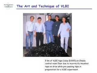
The Art and Technique of VLBI. 5 km of VLBI tape (value $1000) on Onsala control room floor due to incorrectly mounted tape on drive while pre-passing tape in preparation for a VLBI experiment. VLBI Principle. Basic observable: time difference of signal arrival. Global VLBI Stations.

E N D
The Art and Technique of VLBI 5 km of VLBI tape (value $1000) on Onsala control room floor due to incorrectly mounted tape on drive while pre-passing tape in preparation for a VLBI experiment.
VLBI Principle Basic observable: time difference of signal arrival
Global VLBI Stations Geodetic VLBI network + some astronomical stations (GSFC VLBI group)
VLBA Station Electronics At Antenna: ● Select right or left circular polarization ● Add calibration signals ● Amplify ● Mix with local oscillator signal to translate frequency band down to 500 – 1000 MHz for transmission In building: ● Distribute copies of signal to 8 baseband converters ● Mix with local oscillator in BBC to trans- late band to baseband (0.062 – 16 MHz) ● Sample (1 or 2 bit) ● Format for tape ● Record ● Keep time and stable frequency Walker (2002)
Station Electronics: Feed Horn 1. Want linear field shape in aperture for high polarization purity, but modes in circular waveguide are not linear. So, introduce a step to excite two special modes that sum to give a linear field shape 2. Want broad bandwidth, but step 1. works for only one frequency since the two modes propagate at different speeds at different frequencies. So, corrugate the surface to make modes propagate at same speed. 3. Want beamwidth matched to size of telescope, so make aperture as broad as needed. Johnson & Jasik (1984)
Station Electronics: Polarizer One linear comes out here Orthomode transducer (separates polarizations) Other linear comes out here Send orthogonal linear polarizations in here Chattopadhyay et al. (1998) 90◦ hybrid junction (converts linear to circular polarization) Signal 1 + e-i π/4 Signal 2 Signal 1 Signal 2 Signal 2 + e-i π/4 Signal 1 James & Hall (1989)
Station Electronics: Low-Noise Amplifier Metal mounting block Input waveguide Dipole probe into waveguide couples to electric field indium phosphide MMIC Impedance matching network Transistor junctions (amplification happens here) DC voltage supply for transistors Output waveguide 4 stage 100 GHz InP MMIC amplifier (MMIC = monolithic microwave integrated circuit)
Station Electronics: Receiver Feed horns Thermal gap in waveguide Copper straps for heat transport to refrigerator Polarizer Low-noise amplifiers 15 K stage 77 K stage Stirling-cycle refrigerator ATNF multi-band mm-wave receiver
Station Electronics: Downconversion Why? For RG 58 coaxial cable: Loss at 1 GHz = 66 dB / 100 m Dielectric loss ~ frequency 8.4 GHz and 400 m: 10-222 of signal comes out a: Outer plastic sheath b: Copper shield (outer conductor; cylindrical) c: Dielectric insulator d: Copper core (inner conductor) Best cables: air dielectric + bigger diameter -> 2.3 dB / 100 m. But they don't bend much and are expensive. How? Multiply signal by sinusoid at a known, stable frequency ωLO. Generates sum and difference frequencies: A(t) . sin(ωt) . cos(ωLO t) = 2 . A(t) . [sin(ω + ωLO) + sin(ω - ωLO)] Filter off the sum (too high frequency) -> A(t) . sin(ω - ωLO) Send this intermediate frequency (IF) signal down the cable.
Station Electronics: Cable Compensation Cable loss is frequency dependent -> high frequencies have low amplitude Solution: pass signal through a filter with the inverse characteristic, ie large attenuation at low frequencies. Result: relatively flat spectrum for later stages of processing
Station Electronics: IF Distributor IF Distributor: make multiple copies of the IF signal send each to a baseband converter Hybrid power splitter: matches impedance on all ports low loss But: narrow-band Resistive power splitter: matches impedance on all ports compact broad band (DC to GHz) But: factor-of-two loss (ok for IF processing, not ok for RF phasing of antennas)
Station Electronics: Baseband Converter Why downconvert from IF to baseband? ●narrow filters are easier at baseband since fractional bandwidth larger eg 16 MHz filter at 750 MHz = 2 % fractional bandwidth 16 MHz filter at 0 MHz = 200 % fractional bandwidth ●filter centre frequency can be tuned simply by tuning the LO in the BBC ●sampling at baseband is easier Baseband converter (BBC): amplify further downconvert from intermediate frequency (500-1000 MHZ) to zero frequency filter to selectable bandwidth of 16 MHz, 8 MHz, 4 MHz, … 0.0625 MHz Effect: 500 1000 MHz Input IF spectrum 500 1000 MHz Output spectrum band of interest 0 0
Station Electronics: Baseband Converter For small fractional bandwidth need high Q -> large energy stored in filter -> sensitive to temperature -> better to downconvert to baseband to get large fractional bandwidth (Filter design is beyond the scope here; a large and mature field) Recall filters: A simple example (Horowitz & Hill 1989) More complex filter gives steep flanks, excellent stop-band rejection (Horowitz & Hill 1989; telephone filter)
Station Electronics: Baseband Converter Uses two mixers driven by one LO One mixer has 90º phase shift in LO followed by another 90º shift after mix. Result: 180º phase shift of one sideband Summing cancels one sideband. Differencing cancels other sideband. Horowitz & Hill (1989) Standard downconversion: Single-sideband downconversion: (used in BBC) sidebands overlapped -> degrades SNR upper sideband lower sideband LO 0 1000 MHz 500 500 Input IF spectrum 1000 MHz Output spectrum 0
Station Electronics: Sampler Uses multiple comparators, each with its own threshold voltage, looking at the same input signal. Sampler statistics tell whether the thresholds are set correctly. (for 1-bit, want 50% 1’s, 50% 0’s Can servo the thresholds to give the correct statistics, provided input power is within the range of adjustment of thresholds. If not, must change attenuation of input power; routine during setup) Horowitz & Hill (1989) Ladder of resistors gives successively increasing voltages for comparison with the input signal 1-bit sampler: Comparator: Vout = 105 ( V1 – V2) is saturated most of the time Multi-level flash sampler: Input signal
Station Electronics: Formatter Output: VLBA Tape Frame Format (Whitney 1995) Inputs: bit streams from all samplers from all BBCs 5 MHz from maser 1 pulse per second from maser
Station Electronics: Digital BBC Key spectacular development in last few years: field-programmable gate array (FPGA) FPGA = a VLSI chip with huge numbers of logic gates and software- programmable switches to connect them together as you wish. (eg Xilinx Virtex 5: 200 000 flip-flops, 200 000 LUTs, 2 MB RAM, 384 DSPs containing a multiplier, and adder and an accumulator, clock rate 550 MHz. Up to 1200 pins on the package (!) ) Capacity and speed has grown such that analogue radio or TV receivers can now be implemented digitally up to ~ 1 GHz. Analogue replaced by digital Heart of the DBBC: stacked ADC cards and FPGA cards Analogue VLBA terminal (> 20 yr old)
Station Electronics: Digital BBC FPGA core board v1 (circa 2005) 1 core board = 1 BBC Single-sideband conversion to baseband, filters (perfect bandpass shape) Bit-reduction to 1 or 2 bit for recording (no formatter function since newest recorders Mark 5B do not need a formatter) ADC board v1 and v2 developed at MPIfR, core board at Noto 14 layers Stripline transmission lines, impedance matched and equal lengths IF input (eg 500-1000 MHz) analogue-to-digital converter card v1 outputs 8 bits/sample, 1 Gsample/s Digital data flow 8 Gbps per IF (!) to recorder
Station Electronics: Recorder 2003 Mark 5A: Direct replacement for tape recorders, time is in headers from formatter. Data input via same connector as used for tape drives, Records tracks from formatter,up to 1 Gbps Mark 5B: Introduced VSI-H connector, 32 bit parallel data in. Formatterless. Time comes from external 1 pps input, high-order time from PC clock. Disk frame headers are inserted by Mark 5B every 104 bytes, containing time calculated by counting samples since latest 1 pps 2008 Mark 5C: Data I/O via 10 Gbps ethernet at 4 Gbps; a packet recorder Mark 5 disk-based recorder Records 1 Gbps for 18 h unattended Commercial off-the-shelf PC components Prototype worked 3 months from project start Developed starting 2001.
Station Electronics: Recorder: A Paradox Burke (1969) Nature Two element interferometer is a Young's double slit Each photon passes through both antennas (slits) The Paradox: VLBI records signal for later playback So, play back once and get fringes play back a second time and count photon arrivals at slit The Resolution: Amplifier must add noise > hv/k (>> signal) Signal phase preserved and can't count signal photons
Station Electronics: Time and Frequency Standard hydrogen maser – hydrogen maser hydrogen maser – rubidium EVN June 2005, project EI008 Torun H-maser failed and was away for repair
Station Clock A commercial rubidium standard An EFOS hydrogen maser with covers removed (Neuchatel) Stability: 3x10-15 over 1000 s (1 s in 107 yr) 1x10-12 over 1000 s Cost: ~ 200 kEUR (!) ~ 5 kEUR Manufacturers: Smithsonian Astrophysical Observatory (USA) Observatoire de Neuchatel (Switzerland) Sigma Tau (now Symmetricom) (USA) Communications Research Lab (Japan) Vremya-CH (Russia) KVARTZ (Russia)
Station Clock: Hydrogen Maser (H2 -> H + H) (TE011 cavity tuned to 1420 MHz) Output is extremely stable due to: ●long atomic storage time (1 s) gives narrow resonance line ●no wall relaxation (teflon coating) Humphrey et al. (2003)
Station Clock: Stability is not Accuracy eg: H maser Rubidium Caesium Optical (?) eg: H maser Rubidium Caesium Optical (?) (Illustration from Percival, Applied Microwave & Wireless, 1999)
Station Clock: Rate and Drift Effelsberg maser – GPS time, April 2005 0.5 μs (EFOS hydrogen maser from Obs. Neuchatel) 1 month (= 3x10¹²μs) Rate = 0.5 μs / 3x10¹²μs = 1.7x10⁻¹³ s/s Compare to correlator delay window: ~ 1 μs Drift due to cavity frequency change (due temperature, ...)
Future: Optical Time & Frequency Standards? Gill & Margolis Physics World May 2005
Optical Clock: Ion Trap Paul trap: ring electrode, 1.3 mm diameter and end caps Crystal of five stored 172Yb+ ions (fluorescence emission) Physikalisch-Technisch Bundesanstalt (PTB) - Germany
Station Electronics: LO Generation Problem: maser outputs a sinusoid at 5 MHz mixer requires a sinusoid at, eg, 1000 MHz, tunable, phase locked to maser. Solution: phase-locked loop synthesizer. Principle: phase detector 5 MHz ref. from maser low-pass filter gain voltage- controlled oscillator divide by n n x 5 MHz output
Station Electronics: LO Generation Applied magnetic field aligns electron spins, causes Zeeman splitting. Oscillator drives Larmor precession at a frequency dependent on applied magnetic field (2.8 MHz/gauss) (electron spin resonance) Oscillator frequency is tuned via the magnetic field strength Q = thousands; spectrally pure; octave tuning ranges Divide by n: eg, a binary counter, reset to zero when reaching n. Many variants: offset loops, locking to harmonic of reference Key performance: phase noise, capture and lock range, lock speed VCO: eg, yttrium iron garnet (YIG) oscillator Kaa (2004) garnet sphere RF coupling coil Phase detector: Horowitz & Hill (1989)
Station Electronics: Cable Length Calibration Problem: maser is in control room but LO and mixer are in receiver room Cable joining the two is stretched during antenna motion and is heated by sun, both changing the electrical length, hence adding phase noise to LO. Solution: Measure the cable length by sending up a tone and reflecting some back and measure the round-trip phase (aka ‘Cable Cal’)
Station Electronics: Amplitude Calibration Method: monitor total power in IF (written in station log) inject known noise from a noise diode into front end compare resulting step in IF power to the system noise ratio of step sizes = Tcal/Tsys If Tcal is known, this gives Tsys To measure Tcal: perform on-off on primary calibrator switch noise diode on/off ratio of step sizes gives Tcal / Tsource Problem: How can you measure source amplitudes when 1 bit sampling throws away ampitude information !? Hint 1: Correlation coefficient from correlator measures degree of similarity of signals from the two antennas. Hint 2: Signal from a point source is 100 % correlated at the two stations. Hint 3: Noise from the receivers is completely uncorrelated. Solution: Measure the system noise and the SNR (correlation coefficient) and you’ve got enough to derive the signal strength.
Ship Data to Correlator 2000 GB / 3 days = 60 Mbps Price: ~ 50 EUR to 150 EUR
Correlator ● Play back disks or tapes ● Synchronize data to ns level ● Delay the signals according to model ● Correct Doppler shift due Earth rotation ● Cross correlate (-> lag spectrum) ● Fourier transform (lag spectrum -> frequency spectrum) ● Average many spectra for 0.1 s to 10 s ● Write data to output data file for post processing (Covered earlier by Walter Alef) JIVE Correlator, Dwingeloo, NL For EVN production correlation MPIfR/BKG Correlator, Bonn VLBA Correlator, Socorro, USA USNO Correlator, Washington Haystack Correlator Mitaka Correlator, Japan LBA Correlator, Sydney, Australia Penticton Correlator, Canada
Correlator: Delay Model (CALC) BKG Sonderheft “Earth Rotation” (1998) Adapted from Sovers et al. (1998) by Walker (1998)
A Single Correlator Single-sample delays (shift register) Antenna 1 -> Antenna 2 -> XOR Σ Lag Spectrum: correlation coefficient x 106 Time lag (channels) Romney (1998)
Post Processing: Transform from Lag to Frequency Lag Spectrum: correlation coefficient x 106 Time lag (channels) Fourier Transform Frequency Spectrum: phase amplitude Frequency (channels)
Post Processing: Raw Residual Data Phase slope in time is “fringe rate” Phase slope in frequency is delay Frequency channel Frequency channel Walker (2002)
Post Processing: Effect of a Delay Error phase: φ1 = 2π τ v phase: φ2 = φ1+ dφ = 2π τ (v + dv) Path length = L Delay τ = L / c Phase difference: φ2 – φ1 = dφ = 2 π τ dν dφ / dν = 2 π τ A gradient of phase with frequency indicates a delay error
Geodetic VLBI: Polar Motion 3 m 1.1.1991 17.7.1995 500 mas Two components: 1.0 yr period “annual component” 1.18 yr period “Chandler wobble” discovered in 1891, explained in 2000: Fluctuating pressure at ocean bottom due to temperature and salinity changes, wind-driven change in ocean circulation and atmospheric pressure fluctuations (Gross 2000, Geophys. Res. Lett.) BKG Sonderheft “Earth Rotation” (1998)
Geodetic VLBI: Polar Motion Pole y coordinate after subtracting the Chandler component Equatorial component of the atmospheric angular momentum Polar motion is affected by distribution of atmosphere in addition to oceans BKG Sonderheft “Earth Rotation” (1998)
Geodetic VLBI: Length of Day Variations 1 ms/day = 0.46 m/day = 15 mas/day (Vrotation = 465 m/s at equator) Subtract Chandler variation from Length of Day: Length of day Length of day and atmospheric angular momentum are highly correlated: LoD is affected by wind Atmospheric angular momentum BKG Sonderheft “Earth Rotation” (1998)
Earth Orientation Parameter Errors and Spacecraft Navigation Mars Reconnaissance Orbiter Launched 12 Aug, 2005 Cameras & spectrometers for mineral analysis Ground-penetrating radar for sub-surface water ice $500 million spacecraft cost Arrived at Mars March, 2006
Earth Orientation Parameter Errors and Spacecraft Navigation 1.6 x 10⁹ km This angle gives Mars Reconnaissance Orbiter position Mars 105 +/- 15 km MRO Length of Day affects telescope position 1 ms/day = 0.46 m/day at earth equator = 27 km/day at Mars Altitude for mars orbit insertion = 300 km Altitude for aerobraking = 105 +/- 15 km 1 to 5 days without measuring LOD -> error > altitude tolerance -> Mars Reconnaissance Orbiter would burn up or miss Mars
EOP and Ocean Tides Influence of ocean tide on UT1 VLBI measurements Tide model 1 – 10 January 1995 Influence of ocean tide on pole position 2 mas 0 ms Ocean tide (O1) and zonal tide (M2) (periods ~ 12 h) -2 mas BKG Sonderheft “Earth Rotation” (1998)
Station Positions and Continental Drift 1999 1984 30 cm Baseline length Westford-Wettzell 1 – 10 January 1995 Component perpendicular to baseline 20 cm ● Continental drift is clear ● Precision of baseline measurement improves with time GSFC VLBI group (Jan 2000 solution)
Station Positions and Continental Drift 1 – 10 January 1995
Astrometry: Galactic Centre VLBA, 43 GHz inverse-phase referencing to nearby weak calibrator 15 s source changes Galactic rotation: 219 km/s Mass Sgr A*: > 10 % of 4x10⁶ Msun No binary companion > 104 Msun Reid & Brunthaler (2004)
Astrometry: Local Group Motions VLBA, 22 GHz, water masers, phase referencing 1 min cycle, tropospheric delay calibration M33/19 proper motion Brunthaler, Rector, Thilker, Braun (2006) Brunthaler (2006)