Download
1 / 19
190 likes | 315 Views
This presentation discusses the statistical performance analysis of scientific applications on supercomputers, focusing on identifying causes of slow execution, such as improper memory usage and inadequate parallelism. It emphasizes the use of profiling tools (like FPMPI and PAPI) for comprehensive performance reports and proposes a framework to analyze HPC benchmarks. By applying statistical methods and variable clustering, the goal is to extract meaningful performance indices that guide users in optimizing their applications. The implications for diverse scientific applications, including molecular dynamics and weather forecasting, are also highlighted.

E N D
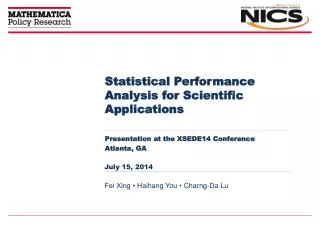
Statistical Performance Analysis for Scientific Applications Fei Xing • Haihang You • Charng-Da Lu July 15, 2014 Presentation at the XSEDE14 Conference Atlanta, GA
Running Time Analysis • Causes of slow run on supercomputer • Improper memory usage • Poor parallelism • Too much I/O • Not optimize the program efficiently • … • Examine user’s code: profiling tools • Profiling = physical exam for applications • Communication – Fast Profiling library for MPI (FPMPI) • Processor & memory – Performance Application Programming Interface (PAPI) • Overall performance & Optimization opportunity – CrayPat
Profiling Reports • Profiling tools produce comprehensive reports covering a wider spectrum of application performance • Imagine, as a scientist and supercomputer user, you see… • Question: how to make sense of these information from the report? • Meaning of the variables • Indication of the numbers TLB miss L1 Cache access MPI communication imbalance MPI calls MPI synchronization time Memory usage MPI communication time Level 1 Cache miss I/O write time MPI imbalance I/O read time More are coming!!!
Research Framework • Select an HPC benchmark to create baseline kernels • Use profiling tools to capture the peak performance • Apply statistical approach to extract synthetic features that are easy to interpret • Run real applications, and compare their performance with “role models” How about… Courtesy of C.-D. Lu
Gears for the Experiment • Benchmarks – HPC Challenge (HPCC) • Gauge supercomputers toward peak performance • 7 representative kernels: • DGEMM, FFT, HPL, Random Access, PTRANS, Latency Bandwidth, Stream • HPL is used in the TOP 500 ranking • 3 parallelism regimes • Serial / Single Processor • Embarrassingly Parallel • MPI Parallel • Profiling tools – FPMPI and PAPI • Testing environment – Kraken (Cray XT5)
HPCC Mode 1 means serial/single processor, * means embarrassingly parallel, M means MPI parallel
Training Set Design • 2,954 observations • Various kernels, wide range of matrix sizes, different compute nodes • 11 performance metrics – gathered from FPMPI and PAPI • MPI communication time, MPI synchronization time, MPI calls, total MPI bytes, memory, FLOPS, total instructions, L2 data cache access, L1 data cache access, synchronization imbalance, communication imbalance • Data preprocessing • Convert some metrics to unit-less rates: divide by wall-time • Normalization Performance Metrics Obs.
Extract Synthetic Features • Extract synthetic & accessible Performance Indices (PIs) • Solution: Variable Clustering + Principal Component Analysis (PCA) • PCA: decorrelate the data • Problem of using PCA alone: variables with small loadings may over influence the PC score • Standardization & modified PCA do not work well
Variable Clustering • Given a partition of X, Pk = (C1, …, Ck) • Centroid of cluster Ci • is the Pearson Correlation • is 1st Principle Component of Ci • Homogeneity of Ci • Quality of clustering , is • Optimal partition
Variable Clustering – Visualize This! • Optimal partition: Given a partition: P4= (C1, …, C4) Centroid of Ck: 1st PC of Ck Quality of P4: = H(C1) + H(C2) + H(C3) + H(C4)
Implementation • Theoretical optimum is computationally complex • Agglomerative hierarchical clustering • Start with the points as individual clusters • At each step, merge the closest pair of clusters until only one cluster left • Result can be visualized as a dendrogram • ClustOfVar in R
Simulation Output PI3: Computation + + + + + + + + 0.53* 0.52* 0.46* 0.49* 1.00* -0.07* -0.15* 0.81* -0.30* -0.14* 0.45* PI2: Memory PI1: Communication
PI1 vs PI2 • 2 distinct strata on memory • Upper – multiple node runs, need extra memory buffers • Lower – single node runs, shared memory • High PI2 for HPL PI2. Memory PI1. Communication
PI1 vs PI3 • Similar PI3 pattern for HPL and DGEMM • Computation intensive • HPL utilize DGEMM routine extensively • Similar all PIs for stream & random access PI3. Computation PI1. Communication
Applications Voronoi Diagram • 9 real-world scientific applications in weather forecasting, molecular dynamics and quantum physics • Amber: molecular dynamics • ExaML: molecular sequencing • GADGET: cosmology • Gromacs: molecular dynamics • HOMME: climate modeling • LAMMPS: molecular dynamics • MILC: quantum chromodynamics • NAMD: molecular dynamics • WRF: weather research PI3. Computation PI1. Communication
Conclusion and Future Work We have • Proposed a statistical approach to give users a better insights into massive performance datasets; • Created a performance scoring system using 3 PIs to capture high-dimensional performance space; • Gave user accessible performance implications and improvement hints. We will • Test the method on other machine and systems; • Define and develop a set of baseline kernels that better represent HPC workloads; • Construct a user-friendly system incorporating statistical techniques to drive more advanced performance analysis for non-experts.
Thanks for your attention! Questions?