Download
1 / 99
1.02k likes | 1.21k Views
Advanced Differential Expression Analysis. Outline. Review of the basic ideas Introduction to (Empirical) Bayesian Statistics The multiple comparison problem SAM. Quantifying Differentially Expression. Two questions.

E N D
Outline • Review of the basic ideas • Introduction to (Empirical) Bayesian Statistics • The multiple comparison problem • SAM
Two questions • Can we order genes by interest? One goal is to assign a one number summary and consider large values interesting. We will refer to this number as a score • How interesting are the most interesting genes? How do their scores compare to the those of genes known not to be interesting?
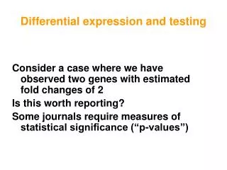
Example • Consider a case were we have observed two genes with fold changes of 2 • Is this worth reporting? Are they both as interesting? Some journals require statistical significance. What does this mean? * *
Review of Statistical Inference • Let Y-X be our measurement representing differential expression. • What is the typical null hypothesis? • P-value is Prob(Y-X as extreme under null) and is a way to summarize how interesting a gene is. • Popular assumption: Under the null,Y-X follows a normal distribution with mean 0 and standard deviation . • Without we do not know the p-value. • We can estimate by taking a sample and using the sample standard deviations. Note: Different genes have different ,
Sample Summaries Observations: Averages: SD2 or variances:
The t-statistic t - statistic:
Properties of t-statistic • If the number of replicates is very large the t-statistic is normally distributed with mean 0 and and SD of 1 • If the observed data, i.e. Y-X, are normally distributed then the t-statistic follows a t distribution regardless of sample size • With one of these two we can compute p-values with one R command
Problems • Problem 1: T-statistic bigger for genes with smaller standard errors estimates • Implication: Ranking might not be optimal • Problem 2: T-statistic not t-distributed. • Implication: p-values/inference incorrect
Problem 1 • With few replicates SD estimates are unstable • Empirical Bayes methodology and Stein estimators provides a statistically rigorous way of improving this estimate • SAM, a more ad-hoc procedure, works well in practice Note: We won’t talk about Stein estimators. See a paper by Gary Churchill for details
Problem 2 • Even if we use a parametric model to improve standard error estimates, the assumptions might not be good enough to provide trust-worthy p-values • We will describe non-parametric approaches for obtaining p-values Note: We still haven’t discussed the multiple comparison problem. That comes later.
Outline • General Introduction • Models for relative expression • Models for absolute expression
Borrowing Strength • An advantage of having tens of thousands of genes is that we can try to learn about typical standard deviations by looking at all genes • Empirical Bayes gives us a formal way of doing this
Modeling Relative Expression Courtesy of Gordon Smyth
Hierarchical Model Normal Model Prior Reparametrization of Lönnstedt and Speed 2002 Normality, independence assumptions are wrong but convenient, resulting methods are useful
Posterior Statistics Posterior variance estimators Moderated t-statistics Eliminates large t-statistics merely from very small s
Marginal Distributions The marginal distributions of the sample variancesand moderated t-statistics are mutually independent Degrees of freedom add!
Shrinkage of Standard Deviations The data decides whether should be closer to tg,pooled or to tg
Posterior Odds Posterior probability of differential expression for any gene is Monotonic function of for constant d Reparametrization of Lönnstedt and Speed 2002
Modeling the Absolute Expression Courtesy of Christina Kendziorski
Hierarchical Model for Expression Data (Two conditions) • Let denote data (one gene) in conditions C1 and C2. • Two patterns of expression: P0 (EE) : P1 (DE): • For P0, • For P1,
=> => Hierarchical Mixture Model for Expression Data • Two conditions: • Multiple conditions: • Parameter estimates via EM • Bayes rule determines threshold here; could target specific FDR.
For every transcript, two conditions => two patterns (DE, EE) EE: m1= m2 DE: m1 m2 Empirical Bayes methods make use all of the data to make gene specific inferences.
Comments on Empirical Bayes Approach(EBarrays) • Hierarchical model is used to estimate posterior probabilities of patterns of expression. The model accounts for the measurement error process and for fluctuations in absolute expression levels. • Multiple conditions are handled in the same way as two conditions (no extra work required!). • Posterior probabilities of expression patterns are calculated for every transcript. • Threshold can be adjusted to target a specific FDR. • In Bioconductor
Empirical Bayes for Microarrays (EBarrays) On Differential Variability of Expression Ratios: Improving Statistical Inference About Gene Expression Changes from Microarray Data by M.A. Newton, C.M. Kendziorski, C.S. Richmond, F.R. Blattner, and K.W. Tsui Journal of Computational Biology 8: 37-52, 2001. On Parametric Empirical Bayes Methods for Comparing Multiple Groups Using Replicated Gene Expression Profiles by C.M. Kendziorski, M.A. Newton, H. Lan and M.N. Gould Statistics in Medicine, to appear, 2003.
Inference and the Multiple Comparison Problem Many slides courtesy of John Storey
Once you have a given score for each gene, how do you decide on a cut-off? p-values are popular. But how do we decide on a cut-off? Are 0.05 and 0.01 appropriate? Are the p-values correct? Hypothesis testing
P-values by permutation • It is common for the assumptions used to derive the statistics used to summarize interest are not approximate enough to yield useful p-values • An alternative is to use permutations
p-values by permutations We focus on one gene only. For the bth iteration, b = 1, , B; Permute the n data points for the gene (x). The first n1 are referred to as “treatments”, the second n2 as “controls”. For each gene, calculate the corresponding two sample t-statistic, tb. After all the B permutations are done; Put p = #{b: |tb| ≥ |tobserved|}/B (p lower if we use >).
Multiple Comparison Problem • If we do have useful approximations of our p-values, we still face the multiple comparison problem • When performing many independent tests p-values no longer have the same interpretation
Hypothesis Testing • Test for each gene null hypothesis: no differential expression. • Two types of errors can be committed • Type I error or false positive (say that a gene is differentially expressed when it is not, i.e., reject a true null hypothesis). • Type II error or false negative (fail to identify a truly differentially expressed gene, i.e.,fail to reject a false null hypothesis)
Multiple Hypothesis Testing • What happens if we call all genes significant with p-values ≤ 0.05, for example? Null = Equivalent Expression; Alternative = Differential Expression
Other ways of thinking of P-values • A p-value is defined to be the minimum false positive rate at which an observed statistic can be called significant • If the null hypothesis is simple, then a null p-value is uniformly distributed
Multiple Hypothesis TestError Controlling Procedure • Suppose m hypotheses are tested with p-values p1, p2, …, pm • A multiple hypothesis error controlling procedure is a function T(p; ) such that rejecting all nulls with pi≤ T(p; ) implies that Error≤ • Error is a population quantity (not random)
Weak and Strong Control • If T(p; ) is such Error≤ only when m0 = m, then the procedure provides weak control of the error measure • If T(p; ) is such Error≤ for any value of m0, then the procedure provides strong control of the error measure – note that m0 is not an argument of T(p; )!
Error Rates • Per comparison error rate (PCER): the expected value of the number of Type I errors over the number of hypotheses PCER = E(V)/m • Per family error rate (PFER): the expected number of Type I errors PFER = E(V) • Family-wise error rate: the probability of at least one Type I error FEWR = Pr(V ≥ 1) • False discovery rate (FDR) rate that false discoveries occur FDR = E(V/R; R>0) = E(V/R | R>0)Pr(R>0) • Positive false discovery rate (pFDR): rate that discoveries are false pFDR = E(V/R | R>0).