Download
1 / 35
360 likes | 509 Views
Factorial ANOVA. More than one categorical explanatory variable. Factorial ANOVA. Categorical explanatory variables are called factors More than one at a time Originally for true experiments, but also useful with observational data

E N D
Factorial ANOVA More than one categorical explanatory variable
Factorial ANOVA • Categorical explanatory variables are called factors • More than one at a time • Originally for true experiments, but also useful with observational data • If there are observations at all combinations of explanatory variable values, it’s called a complete factorial design (as opposed to a fractional factorial).
The potato study • Cases are storage containers (of potatoes) • Same number of potatoes in each container. Inoculate with bacteria, store for a fixed time period. • Response variable is number of rotten potatoes. • Two explanatory variables, randomly assigned • Bacteria Type (1, 2, 3) • Temperature (1=Cool, 2=Warm)
Two-factor design Six treatment conditions
Factorial experiments • Allow more than one factor to be investigated in the same study: Efficiency! • Allow the scientist to see whether the effect of an explanatory variable depends on the value of another explanatory variable: Interactions • Thank you again, Mr. Fisher.
Tests • Main effects: Differences among marginal means • Interactions: Differences between differences (What is the effect of Factor A? It depends on the level of Factor B.)
Testing Contrasts • Differences between marginal means are definitely contrasts • Interactions are also sets of contrasts
Equivalent statements • The effect of A depends upon B • The effect of B depends on A
Three factors: A, B and C • There are three (sets of) main effects: One each for A, B, C • There are three two-factor interactions • A by B (Averaging over C) • A by C (Averaging over B) • B by C (Averaging over A) • There is one three-factor interaction: AxBxC
Meaning of the 3-factor interaction • The form of the A x B interaction depends on the value of C • The form of the A x C interaction depends on the value of B • The form of the B x C interaction depends on the value of A • These statements are equivalent. Use the one that is easiest to understand.
To graph a three-factor interaction • Make a separate mean plot (showing a 2-factor interaction) for each value of the third variable. • In the potato study, a graph for each type of potato
Four-factor design • Four sets of main effects • Six two-factor interactions • Four three-factor interactions • One four-factor interaction: The nature of the three-factor interaction depends on the value of the 4th factor • There is an F test for each one • And so on …
As the number of factors increases • The higher-way interactions get harder and harder to understand • All the tests are still tests of sets of contrasts (differences between differences of differences …) • But it gets harder and harder to write down the contrasts • Effect coding becomes easier
Interaction effects are products of dummy variables • The A x B interaction: Multiply each dummy variable for A by each dummy variable for B • Use these products as additional explanatory variables in the multiple regression • The A x B x C interaction: Multiply each dummy variable for C by each product term from the A x B interaction • Test the sets of product terms simultaneously
We see • Intercept is the grand mean • Regression coefficients for the dummy variables are deviations of the marginal means from the grand mean • What about the interactions?
Factorial ANOVA with effect coding is pretty automatic • You don’t have to make a table unless asked • It always works as you expect it will • Hypothesis tests are the same as testing sets of contrasts • Covariates present no problem. Main effects and interactions have their usual meanings, “controlling” for the covariates. • Plot the least squares means
Again • Intercept is the grand mean • Regression coefficients for the dummy variables are deviations of the marginal means from the grand mean • Test of main effect(s) is test of the dummy variables for a factor. • Interaction effects are products of dummy variables.
Balanced vs. Unbalanced Experimental Designs • Balanced design: Cell sample sizes are proportional (maybe equal) • Explanatory variables have zero relationship to one another • Numerator SS in ANOVA are independent • Everything is nice and simple • Most experimental studies are designed this way. • As soon as somebody drops a test tube, it’s no longer true
Analysis of unbalanced data • When explanatory variables are related, there is potential ambiguity. • A is related to Y, B is related to Y, and A is related to B. • Who gets credit for the portion of variation in Y that could be explained by either A or B? • With a regression approach, whether you use contrasts or dummy variables (equivalent), the answer is nobody. • Think of full, reduced models. • Equivalently, general linear test
Some software is designed for balanced data • The special purpose formulas are much simpler. • Very useful in the past. • Since most data are at least a little unbalanced, a recipe for trouble. • Most textbook data are balanced, so they cannot tell you what your software is really doing. • R’s anova and aov functions are designed for balanced data, though anova applied to lm objects can give you what you want if you use it with care. • SAS proc glm is much more convenient. SAS proc anova is for balanced data.