Download

1 / 39
390 likes | 495 Views
Learn how ANOVA helps compare multiple groups in research settings, the importance of managing Type I errors, and the Bonferroni correction method. Understand variance, ANOVA tables, and conducting ANOVA in complex experimental designs.

E N D
Conducting ANOVA’s Why? A. more than two groups to compare
Conducting ANOVA’s Why? A. more than two groups to compare What’s the prob? D. putridalow density D. putridahigh density D. putridawith D. tripuncatata
Conducting ANOVA’s Why? A. more than two groups to compare What’s the prob? D. putridalow density D. putridahigh density D. putridawith D. tripuncatata What was our solution?
Conducting ANOVA’s Why? A. more than two groups to compare What’s the prob? D. putridalow density D. putridahigh density D. putridawith D. tripuncatata What was our solution? U U U
What’s the prob? D. putridalow density D. putridahigh density D. putridawith D. tripuncatata Tested each contrast at p = 0.05 Probability of being correct in rejecting each Ho: 1 2 3 0.95 0.95 0.95 U U U
What’s the prob? D. putridalow density D. putridahigh density D. putridawith D. tripuncatata Tested each contrast at p = 0.05 Probability of being correct in rejecting all Ho: 1 2 3 0.95 x 0.95 x 0.95 = 0.86 So, Type I error rate has increased from 0.05 to 0.14 U U U
Probability of being correct in rejecting all Ho: 1 2 3 0.95 x 0.95 x 0.95 = 0.86 So, Type I error rate has increased from 0.05 to 0.14 Hmmmm….. What can we do to maintain a 0.05 level across all contrasts?
Probability of being correct in rejecting all Ho: 1 2 3 0.95 x 0.95 x 0.95 = 0.86 So, Type I error rate has increased from 0.05 to 0.14 Hmmmm….. What can we do to maintain a 0.05 level across all contrasts? Right. Adjust the comparison-wise error rate.
Probability of being correct in rejecting all Ho: 1 2 3 0.95 x 0.95 x 0.95 = 0.86 So, Type I error rate has increased from 0.05 to 0.14 Simplest: Bonferroni correction: Comparison-wise p = experiment-wise p/n Where n = number of contrasts. Experient-wise = 0.05 Comparison-wise = 0.05/3 = 0.0167
Probability of being correct in rejecting all Ho: 1 2 3 0.95 x 0.95 x 0.95 = 0.86 So, Type I error rate has increased from 0.05 to 0.14 Simplest: Bonferroni correction: Comparison-wise p = experiment-wise p/n Where n = number of contrasts. Experient-wise = 0.05 Comparison-wise = 0.05/3 = 0.0167 So, confidence = 0.983
Probability of being correct in rejecting all Ho: 1 2 3 0.983 x 0.983 x 0.983 = 0.95 So, Type I error rate is now 0.95 Simplest: Bonferroni correction: Comparison-wise p = experiment-wise p/n Where n = number of contrasts. Experient-wise = 0.05 Comparison-wise = 0.05/3 = 0.0167 So, confidence = 0.983
Conducting ANOVA’s Why? A. more than two groups to compare What’s the prob? - multiple comparisons reduce experiment-wide alpha level. - Bonferroni adjustments assume contrasts as independent; but they are both part of the same experiment…
- Bonferroni adjustments assume contrasts as independent; but they are both part of the same experiment… Our consideration of 1 vs. 2 might consider the variation in all treatments that were part of this experiment; especially if we are interpreting the differences between mean comparisons as meaningful. 1 vs. 2 – not significant 1 vs. 3 – significant. So, interspecific competition is more important than intraspecific competition
- Bonferroni adjustments assume contrasts as independent; but they are both part of the same experiment… Our consideration of 1 vs. 2 might consider the variation in all treatments that were part of this experiment; especially if we are interpreting the differences between mean comparisons as meaningful.
Conducting ANOVA’s Why? A. more than two groups to compare B. complex design with multiple factors - blocks - nested terms - interaction effects - correlated variables (covariates) - multiple responses
Conducting ANOVA’s Why? How? A. Variance Redux Of a population Of a sample
Sum of squares n - 1 S2 =
“Sum of squares” = SS n - 1 S2 = (Sx)2 n = SS S(x2) -
“Sum of squares” = SS n - 1 S2 = (Sx)2 n = SS S(x2) - MS = n - 1
Conducting ANOVA’s Why? How? A. Variance Redux B. The ANOVA Table Source of Variation df SS MS F p
Weight gain in mice fed different diets Group A Group B Group C (Control) (Junk Food) (Health Food) 10.8 12.7 9.8 11 13.9 8.6 9.7 11.8 8 10.1 13 7.5 11.2 11 9 9.8 10.9 10 10.5 13.6 8.1 9.5 10.9 7.8 10 11.5 7.9 10.2 12.8 9.1 Group sums Sx Sx2 (Sx)2/n
Weight gain in mice fed different diets Group A Group B Group C (Control) (Junk Food) (Health Food) 10.8 12.7 9.8 11 13.9 8.6 9.7 11.8 8 10.1 13 7.5 11.2 11 9 9.8 10.9 10 10.5 13.6 8.1 9.5 10.9 7.8 10 11.5 7.9 10.2 12.8 9.1 Group sums Totals Sx 102.8 122.1 85.8 310.7 Sx2 1059.76 1502.41 742.92 3305.09 (Sx)2/n 1056.784 1490.841 736.164 3283.789
Weight gain in mice fed different diets Group A Group B Group C (Control) (Junk Food) (Health Food) 10.8 12.7 9.8 11 13.9 8.6 9.7 11.8 8 10.1 13 7.5 11.2 11 9 9.8 10.9 10 10.5 13.6 8.1 9.5 10.9 7.8 10 11.5 7.9 10.2 12.8 9.1 Group sums Totals Sx 102.8 122.1 85.8 310.7 Sx2 1059.76 1502.41 742.92 3305.09 (Sx)2/n 1056.784 1490.841 736.164 3283.789 Correction term = (SSx)2/N = (310.7)2/30
Weight gain in mice fed different diets Group A Group B Group C (Control) (Junk Food) (Health Food) 10.8 12.7 9.8 11 13.9 8.6 9.7 11.8 8 10.1 13 7.5 11.2 11 9 9.8 10.9 10 10.5 13.6 8.1 9.5 10.9 7.8 10 11.5 7.9 10.2 12.8 9.1 Group sums Totals Sx 102.8 122.1 85.8 310.7 Sx2 1059.76 1502.41 742.92 3305.09 (Sx)2/n 1056.784 1490.841 736.164 3283.789 3217.816 = CT
Weight gain in mice fed different diets Group sums Totals Sx 102.8 122.1 85.8 310.7 Sx2 1059.76 1502.41 742.92 3305.09 (Sx)2/n 1056.784 1490.841 736.164 3283.789 3217.816 = CT Source of Variation df SS MS F p TOTAL 29 (Sx)2 n = SS S(x2) - SStotal = 3305.09 – 3217.816 = 87.274
Weight gain in mice fed different diets Group sums Totals Sx 102.8 122.1 85.8 310.7 Sx2 1059.76 1502.41 742.92 3305.09 (Sx)2/n 1056.784 1490.841 736.164 3283.789 3217.816 = CT Source of Variation df SS MS F p TOTAL 29 87.274 (Sx)2 n = SS S(x2) - SStotal = 3305.09 – 3217.816 = 87.274
Weight gain in mice fed different diets Group sums Totals Sx 102.8 122.1 85.8 310.7 Sx2 1059.76 1502.41 742.92 3305.09 (Sx)2/n 1056.784 1490.841 736.164 3283.789 3217.816 = CT Source of Variation df SS MS F p TOTAL 29 87.274 GROUP 2 65.973 (Sx)2 n = SS S(x2) - SSgroup = 3283.789 – 3217.816 = 65.973
Weight gain in mice fed different diets Group sums Totals Sx 102.8 122.1 85.8 310.7 Sx2 1059.76 1502.41 742.92 3305.09 (Sx)2/n 1056.784 1490.841 736.164 3283.789 3217.816 = CT Source of Variation df SS MS F p TOTAL 29 87.274 GROUP 2 65.973 32.986 (Sx)2 n S(x2) - MS = MSgroup = 65.973/2 = 32.986 n - 1
Weight gain in mice fed different diets Group sums Totals Sx 102.8 122.1 85.8 310.7 Sx2 1059.76 1502.41 742.92 3305.09 (Sx)2/n 1056.784 1490.841 736.164 3283.789 3217.816 = CT Source of Variation df SS MS F p TOTAL 29 87.274 GROUP 2 65.973 32.986 “ERROR” (within) 27 21.301
Weight gain in mice fed different diets Group sums Totals Sx 102.8 122.1 85.8 310.7 Sx2 1059.76 1502.41 742.92 3305.09 (Sx)2/n 1056.784 1490.841 736.164 3283.789 3217.816 = CT Source of Variation df SS MS F p TOTAL 29 87.274 GROUP 2 65.973 32.986 “ERROR” (within) 27 21.301 0.789 MSerror = 21.301/27 = 0.789
Weight gain in mice fed different diets Group sums Totals Sx 102.8 122.1 85.8 310.7 Sx2 1059.76 1502.41 742.92 3305.09 (Sx)2/n 1056.784 1490.841 736.164 3283.789 3217.816 = CT Source of Variation df SS MS F p TOTAL 29 87.274 GROUP 2 65.973 32.986 “ERROR” (within) 27 21.301 0.789 Variance (MS) between groups Variance (MS) within groups F =
Weight gain in mice fed different diets Group sums Totals Sx 102.8 122.1 85.8 310.7 Sx2 1059.76 1502.41 742.92 3305.09 (Sx)2/n 1056.784 1490.841 736.164 3283.789 3217.816 = CT Source of Variation df SS MS F p TOTAL 29 87.274 GROUP 2 65.973 32.986 41.81 “ERROR” (within) 27 21.301 0.789 32.986 0.789 F = = 41.81
Weight gain in mice fed different diets Group sums Totals Sx 102.8 122.1 85.8 310.7 Sx2 1059.76 1502.41 742.92 3305.09 (Sx)2/n 1056.784 1490.841 736.164 3283.789 3217.816 = CT Source of Variation df SS MS F p TOTAL 29 87.274 GROUP 2 65.973 32.986 41.81 < 0.05 “ERROR” (within) 27 21.301 0.789 32.986 0.789 F = = 41.81
Conducting ANOVA’s Why? How? Comparing Means “post-hoc mean comparison tests – after ANOVA TUKEY – CV = q MSerror n = 0.9915 Q from table A.7 = 3.53 n = n per group (10)
Means: Health Food 8.58 Control 10.29 Junk Food 12.25 H – C = 1.70 J – C = 1.93 H – J = 3.67 All greater than 0.9915, so all mean comparisions are significantly different at an experiment-wide error rate of 0.05.
Means: Health Food 8.58 a Control 10.29 b Junk Food 12.25 c H – C = 1.70 J – C = 1.93 H – J = 3.67 All greater than 0.9915, so all mean comparisions are significantly different at an experiment-wide error rate of 0.05.