Download
1 / 30
300 likes | 327 Views
The IceCube neutrino observatory is a cutting-edge project under construction in Antarctica, designed to detect high-energy neutrinos from cosmic sources like supernovae. This seminar presentation by Kael Hanson from the University of Wisconsin delves into the technical aspects, operational features, and potential scientific implications of using IceCube for supernova detection.

E N D
Detecting Supernovae with IceCube Kael Hanson University of Wisconsin HEP Seminar March 26, 2007
Overview • The IceCube neutrino observatory is currently under construction at the South Pole. To date approximately 30% of the detector is installed and over 50% of the instrumentation has been produced. • Science operation begins 4/1/2007 • As a UHE telescope, IceCube is gigaton detector with effective area in excess of 1 km2 to > TeV muons. • First proposed by Jacobsen, Halzen, Zas PRD 49 (1994), possibility to use background counting of optical detectors for detection of MeV-scale neutrinos from galactic supernovae. • This technique utilized by AMANDA detector since 1998. • With est. 3 Mton effective volume for low-energy ν,IceCube potentially provides detailed information for modeling supernovae: • Bigger, better, lower-noise optical detectors • Data acquisition at fine timescales - 1.6 ms / bin • Supernova detection would provide high resolution, high statistics data for supernova burst models. • Sensitivity may be sufficient for particle physics investigations
The IceCube UHE Neutrino Observatory Both representations not to scale - nevertheless nicely illustrate salient detector characteristics.
IceCube UHE Neutrino Observatory (2) • 1st string deployed Jan-2005 • Last string deployed Jan-2011 • 4500 deep-ice optical modules along 75 strings • Depth ranges 1450 m - 2450 m with 17 m spacing. • 320 surface modules in 80 stations - IceTop • Detector is hybridizing already - this year radio and acoustic test modules deployed and are working well. • IceCube optimized for detection of TeV and PeV-scale neutrinos of cosmic origin: point sources, diffuse HE neutrinos, GRBs, &c.
IceCube Integrated Volume (Projected) • Graph shows cumulative km3·yr of exposure × volume • # of strings per year is based on latest “best guess” deployment rate of 12 strings 2007 (13) and 14 strings per season thereafter. • 1 km3·yr reached 2 years before detector is completed • Close to 4 km3·yr at the beginning of 2nd year of full array operation.
AMANDA • 677 analog OMs deployed along 19 strings • 10 strings 1997 (AMANDA B10) • 3 strings 1998 (AMANDA B13) • 6 strings 2000 (AMANDA II) AMANDA supernova analyses typically employ between 400-500 of these channels due to instabilities in some. • Analog PMT signals using electrical and optical transmission lines. • 200 m diameter, 500 meters height; AMANDA II encompasses 20 Mton instrumented ice volume: 6 times more dense than IceCube. • AMANDA will remain operational and form IceCube Inner Core Detector for low E physics (~ 100 GeV - WIMPs, &c) • IceCube surrounding strings provide effective veto – lower background and can push AMANDA energy threshold down. • Conventional TDC / ADC technology for AMANDA has been entirely replaced by TWR system. • Beginning 2007 season, AMANDA / IceCube data streams are conjoined; detector subsystems will share trigger information.
Optical Properties of Glacial Ice Why deploy in ice? Deep glacial ice is optically transparent. Two mechanisms: scattering length ~ 20 m, absorption ~ O(100) m. Ice has several layers of dust from prehistoric events. Monte Carlo detector simulation must account for this. Reconstruction methods involving maximum likelihood tests against hypotheses have been developed to overcome difficulties posed by photon scattering. Plots above from in situ measurements using artificial light sources in AMANDA. “Hole ice” around deployed modules must also be taken into account.
The Enhanced Hot Water Drill (EHWD) EHWD designed to drill a 2450 m × 60 cm hole in ~30 hr. Fuel budget is 7200 gal per hole. Shown above is drill camp and tower site (inset), both mobile field arrays. Everything must fit into LC-130 for transport to Pole. Supply: 200 GPM @ 1000 psi, 190 °FReturn: 192 GPM @ 33 °F Make-Up: 8 GPM @ 33 °F Thermal Power: 4.5 Megawatt
Drilling Ted Schultz Top layer of packed snow is called firn. Hot water drill designed for ice drilling – it gets starter hole from firn drill (lower right). (Top left and top right) EHWD drill head entering hole.
2005, 2006, 2007 Deployments 80 79 78 77 74 73 72 71 67 66 65 64 59 58 57 56 55 50 49 48 47 46 40 39 38 30 29 21 AMANDA 2005 - 1 string 2006 - 8 strings 56 2007 - 13 strings! IceTop only 2007 1424 DOMs deployed to date1320 DOMs on 22 deep ice strings>99% DOM survival rate Following deployment years will target ≥ 14 strings / year until a ~75 strings are installed. Final detector will include ~4500 in-ice optical modules and 500 surface modules.
The IceCube Digital Optical Module (DOM) DOM Highlights - Optical Large Area Photocathode10” (500 cm2) Hamamatsu R7081-02 bialkali PMT (peak QE 24% @ 420 nm) Low noise< 300 Hz background counting rate in-ice (with deadtime - see later) Glass / Gel ImprovementsBetter transmission in 330 - 400 nm relative to AMANDA OM Optical calibrationEach DOM is calibrated ε(λ) in the lab to about 7%; in-situ flasher board additionally permits in-ice measurements DOM Highlights - Electronics “Smart” sensor digital technologyVersatile FPGA design with option to expand / change programming at any point in lifecycle. Core of supernova DAQ resides inside DOM itself. Array TimingHandled in DOM logic - DOM-to-DOM timing good to 2-3 ns using RAPCal method. Low power - 3.75 W / DOM The DOM has been in production at UW, DESY-Zeuthen, and Stockholm since mid-2004 with very little change. It has met or exceeded design requirements, and, despite harsh re-freeze conditions 2500 m deep, we’ve lost < 0.5 % of the units during this critical phase. To date, 3000 of approx. 5000 units have been produced.
Reducing Background Counting - Deadtime Correlated noise in PMTs Measurements counting all PMT pulses in deployed DOMs yield average rate of approx. 700 Hz / module. Study of the time structure of this noise clearly indicates correlated noise patterns: PMT AfterpulsesWell-known that ionized residual gases in PMTs cause afterpulses on timescale (for large PMTs) of 6-10 µs. Glass ScintillationSmall contamination of rare-earth oxides produces further tail out to 100’s of µs due to scintillation processes. To reduce noise rate and restore Poissonian behavior to fluctuations ,it is necessary to apply afterpulse inhibit (deadtime) when pulse counting. Analysis of real data demonstrates that 200 µs afterpulse suppression window reduces background by factor of 4 while sacrificing only few percent of signal.
DOM Temperatures in the Ice One DOM didn’t freeze-in until May!
Singles Counting Rates vs. Depth Importance of noise rates: 1.) noise rate w/o dead time: 700 Hz, important for DAQ bandwidth 2.) noise rate w/suppression of 50µs: 300Hz, important for event reconstruction and in particular for supernova sensitivity. Two Icecube strings equivalent or more sensitive than all of AMANDA to SN.
The Supernova DAQ In the ice - counting FPGAIntegrate into 1.6384 ms (216 / 40 MHz) bins SPE/MPE discriminator crossings with application of 200 µs deadtime. This counting operation executes in parallel with digitization and readout activity of main DAQ core and does not depend on its state. CPUInterrupted every 6.5 ms (4 bins). Bins are timestamped with ~ 10 ns precision and copied into SDRAM where they await ~1 Hz commands from surface to readout accumulated bins. At the surface - assembly Surface DAQ for supernova is 2-stage assembly of disparate data packets from individual DOM channels: StringHubIssue periodic readouts to string of 60 DOMs. Use RAPCal information to translate DOM timestamps to UTC then perform merge and sort into single stream of data which is sent downstream. SupernovaBuilderFurther merge-and-sort of StringHub streams into final stream written to tape. Began supernova-mode data-taking last September with 9-string 540-module detector. This year’s run is set to begin 5/1. Taking full supernova data (1 MB/sec) since 3/18.
The Online Trigger and the SNEWS Connection Real-time detection of SNe SNEWS and AMANDA Don’t stop there: real-time detection and reporting of burst candidates gives “heads-up” to optical observers. In addition, combining many, distributed observatories makes more sensitive, robust alert. SuperNova Early Warning System [NJP 6 (2004)114] … Strict requirement that individual detector produce no more than 1 false alarm / week. AMANDA official participant since 6/2005. Near real-time delivery of alerts possible through Iridium link to pole (24/7; low-bandwidth) Noise rates in AMANDA can be highly variable. Real-time detection of noisy channels necessary; additionally, detector chi-square reports uniformity of signal in detector (good SN totally uniform). Statistics based on Gaussian approx.; OK for large bins. SNEWS and IceCube Mainz supernova group adapting AMANDA online trigger to handle data feed from IceCube DAQ. Necessary to thoroughly evaluate system to demonstrate that we meet the strict requirement of < 1 false alarm / week. 22-string IceCube will join end of year 2007.
Supernovae • Categorization of SNe historically based on presence of hydrogen in spectroscopic lines: • Type I SNe don’t have it • Type Ia probably from dwarf stars accreting mass to Chandrasekhar limit, then exploding. • Type Ib/c core collapse SNe but have lost hydrogen envelope because of stellar winds (Wolf-Rayet stars) or perhaps mass transfer to companion star. Incidentally, recent investigations associate these types with GRBs (e.g. Woosley and Bloom astro-ph/0609142); variations with slower jets may further be γ dark but still produce TeV ν detectable in IceCube and may be much more common. • Type II SNe have the hydrogen lines - these are likely massive stars with hydrogen envelopes intact that undergo core collapse • Intense neutrino luminosities only with core collapse SNe Type Ib/c and Type II. • Galactic rate of core collapse SNe given by INTEGRAL measurements - 1-3 per century (Nature 439 (2006) 45). Optimistically, given IceCube lifetime of 15 years - 40% chance of observing galactic event.
Core Collapse - Basic Features • Details of physics of core collapse not completely understood due to lack of observational data. 19 neutrino events detected in Kamiokande-II and IMB from SN1987A bolster support for general model but were too few to provide specific insights (see Yuksel and Beacom astro-ph/0702613v2 for recent discussion of SN1987A data). • Massive star (> 8 M⊙)has developed 1.5 M⊙ Fe core which is beginning to neutronize. • “Homologous” core becomes unstable as Fe nuclei leech out electrons and photo-disintegration processes occur and collapses to ~30 km where nuclear repulsion causes ‘core bounce.’ Lots of neutrinos of all flavors inside simmering proto-neutron star. • Shock wave from rebound and collapsing outer portion of core. When shock penetrates “neutrinosphere,” initial neutronization burst escapes. • Core accretes infalling material and begins to radiate ~1053 erg in neutrinos over the next ~ 0.5 s until explosion. • The remainder of the energy is emitted over timescales of 10’s of seconds as the newly-formed neutron star cools • Optical emission some ~10 hr later. • Models still fail, unmanipulated, to provoke explosion - this is continuing mystery which might be unraveled given adequate input data provided by IceCube or future SN neutrino detector.
The Supernova - GRB Connection Ando & Beacom PRL2005 TeV Neutrinos from Nearby SNe GRBs Mounting evidence that Type Ib/c SNe produce GRB. Rate of GRB is 1%. May be many more with mildly relativistic jets (Γ ~ few) which don’t produce significant EM component. TeV neutrinos detectable from nearby objects (D < 20 Mpc) at the rate of ≈ 1 SN / year. [ Razzaque, Mezaros, Waxman PRL (2004) ] SNe ? Sensitivity can be doubled by optical follow-up! MK, A. Mohr, astro-ph/0701618
MeV Supernova Neutrinos in AMANDA 2000-2003 preliminary SN neutrino signal simulation center of galaxy, normalized to SN1987A
MeV Neutrinos in IceCube • Jacobsen, Halzen, Zas PRD 49 (1994) 1758 first proposed. Follow-up calculation for IceCube presented in JCAP 6 (2003) - Dighe, Keil, Raffelt. Unfortunately both groups have some incorrect assumptions. • IceCube supernova analysis group has done preliminary update to IceCube of more detailed work from AMANDA Ph.D. thesis by T. Feser. • Some points from all works: • Neutrino effective volume ∝ E3; 2 powers from σ 1 power from electron/positron tracklength. Thus, detection is sensitive to neutrino energy spectra - or stated another way, effective volumes are all dependent on SN models / oscillations, &c. • Effective volume ∝ Λabsthe optical pathlength in the ice • For SN models this yields approx. 700 m3 Veff- or a sphere around each module of 5 m radius. As such, each module may be treated independently. • Principal detection channel is inverse beta decay (ref cross-sections slide) - this makes detection of neutronization peak difficult. • Currently, with ~ 1300 deep ice modules detector mass is 800 kton. • Full IceCube ~ 4500 modules detector mass 3 Mton.
MeV Neutrinos in IceCube (continued) • The detection comes from increase in background counts across the entire array. • Disadvantages - you have no pointing or energy reconstruction as in Super-K • Advantage is that enormous volume provides high-statistics measurement. Time binning can be made fine. • Signal from 1987A SN at galactic center would produce 475k excess counts in ~10 sec window on a background of 12 ×106 counts from noise - S/N ~ 150:1 in full IceCube; • In current 22-string detector signal is still very significant: 140k excess counts giving S/N ~ 75:1. • Gain comes when decimating signal in time to study time evolution
Signal Predictions From Dighe, et. al. JCAP 06 (2003)005. Note that predicted rate should be scaled dow by 3x - cf. previous slide. Also statistical errors for 50 ms bins are +/- 250 counts. From Dighe, et. al. JCAP 06 (2003)005. Their prediction of earth modulation effect for particular choice of neutrino mixing angle θ13could render IceCube sensitive to neutrino mass hierarchy. IceCube detector sensitive to modulation effect; however, model-dependence of the neutrino luminosity would almost certainly require contemporaneous detection of SN at another detector such as Super-K or Hyper-K.
Detection of neutronization peak Neutronization fluence is largely independent of SN model and progenitor mass - useful as a neutrino standard candle. IceCube detection is marginal.
Neutrino Oscillation in Star From Kachelreiß & Tomàs PRD 71 (2005)
Conclusions • IceCube gigaton high energy neutrino observatory doubles nicely as megaton low energy detector • High-statistics measurements are possible which can at the very least provide detailed measurements of neutrino luminosity vs time. • IceCube longevity gives good chance of observing significant galactic core collapse event. • IceCube is operating and is sensitive to GC events NOW! With 1300 modules deployed in ice this year sensitive to 100% of Milky Way. • SN analysis group working to improve outdated simulations and bring up online supernova trigger • Participation in SNEWS later this year.