Graphs
Graphs. Wolfgang Huber EMBL/EBI Otto-Warburg Summer School Berlin Aug 2005 Based on chapters from "Bioinformatics and Computational Biology Solutions using R and Bioconductor", Gentleman, Carey, Huber, Irizarry, Dudoit. Springer Verlag (2005). Graphs. Set of nodes and set of edges.

Graphs
E N D
Presentation Transcript
Graphs Wolfgang Huber EMBL/EBI Otto-Warburg Summer School Berlin Aug 2005 Based on chapters from "Bioinformatics and Computational Biology Solutions using R and Bioconductor", Gentleman, Carey, Huber, Irizarry, Dudoit. Springer Verlag (2005).
Graphs Set of nodes and set of edges. Nodes: objects of interest Edges: relationships between them A useful abstraction to talk about relationships and interactions (think of integer numbers, apples and fingers) Edges may have weights, directions, types
Practicalities As always, need to distinguish between the true, underlying property of nature that you want to measure, and the actual result of a measurement (experiment) 1. False positive edges 2. False negative edges (were tested, were not found, but are there in nature) 3. Untested edges (were not tested, are not in your data, but are there in nature) Uncertainty is not usually considered in mainstream graph theory, but cannot be ignored in bioinformatics.
Representation From-To matrix Adjacency matrix (straightforward) Adjacency matrix (sparse) Node-edge lists They are equivalent, but may be quite different in performance and convenience for different applications. Can coerce between the representations
Motivating examples Transcription factor graphs Pathway graphs GO Literature graphs Protein-Complex graphs
Transcription factor interactions Nodes = transcription factors Directed edge: X regulates transcription of Y
Transcriptional regulatory networksfrom "genome-wide location analysis" regulator := a transcription factor (TF) or a ligand of a TF tag: c-myc epitope 106 microarrays samples: enriched (tagged-regulator + DNA-promoter) probes: cDNA of all promoter regions spot intensity ~ affinity of a promotor to a certain regulator Lee et al. Science 2002
Transcriptional regulatory network: a bipartite graph 106 regulators (TFs) regulators 6270 promoter regions promoters
Machine-readable pathway databases KEGG reactome BioCarta (biocarta.com) National Cancer Institute cMAP
Gene Ontology (GO) A structed vocabulary to describe molecular function of gene products, biological processes, and cellular components. Plus A set of "is a", "is part of" relationships between these terms Directed acyclic graph
GO graphs >tfG=GOGraph("GO:0003700", GOMFPARENTS)
The bipartite gene-literature graph: actor and event size adjustment actors: genes actor size: number of papers that a gene appears in event: paper event size: number of genes that appear in a paper Example: R. Strausberg et al. Generation and initial analysis of more than 15,000 full-length human and mouse cDNA sequences. PNAS 99:16899–903, 2002 cites 15,000 genes
Closing gene lists with literature Boundary of gene list L: set of all genes that have co-citation (above threshold weight) with genes in L. Gene 1 Gene X Gene 2 Gene 3 Gene Y Gene 4 Gene 5
Graphs: vocabulary Directed, undirected graphs Adjacent nodes Accessible nodes Self-loop Multi-edge Node degree Walk: alternating sequence of nodes and incident edges Closed walk Distance between nodes, shortest walk Trail: walk with no repeated edges Path: trail with no repeated nodes (except possibly first/last) Cycle Connected graph Weakly connected directed graph (see next page)
Graphs: vocabulary Cut: remove edges to disconnect a graph Cut-set: remove nodes - " - Connectivity of a graph Cliques
Bipartite graphs AG adjacency matrix (n x m) of a bipartite graph G with node sets U, V One mode graphs AU = AGt AG AV = AGAGt (Boolean algebra)
Multigraphs Can have different types of edges
Hypergraphs := set of Nodes + set of hyperedges A hyperedge is a set of nodes (can be more than 2) A directed hyperedge: pair (tail and head) of sets of nodes
Directed acyclic graphs Useful for representing hierarchies, partial orderings (e.g. in time, from general to special, from cause to effect) Many applications: GO MeSH Graphical models
Random Edge Graphs n nodes, m edges p(i,j) = 1/m with high probability: m < n/2: many disconnected components m > n/2: one giant connected component: size ~ n. (next biggest: size ~ log(n)). degrees of separation: log(n). Erdös and Rényi 1960
Random edge graph 100 nodes 50 edges degree distribution
Random graphs versus permutation graphs For statistical inference, one can consider null hypotheses based on aforementioned random graph models; and ones based on node permutation of data graphs. The second is often more appropriate.
Cohesive subgroups For data graphs, the concept of clique is usually too restrictive (false negative or untested edges) n-clique: distance between all members is <=n. (Clique: n=1) k-plex: maximal subgraph G in which each member is neighbour of at least |G|-k others. (Clique: k=1) k-core: maximal subgraph G in which each member is neighbour of at least k others. (Clique: k=|G|-1) After: Social Network Analysis, Wasserman and Faust (1994)
Graph layout three different layout engines in (R)graphviz
A Graph Theoretic Algorithm for Estimating ProteinComplex Membership using Data from AffinityPurication - Mass Spectrometry TechnologyDenise Scholtens and Robert Gentleman2004
Two Types of Protein Relationship • AP-MS (Affinity Purification - Mass Spectrometry ) • Measures Complex Comembership • Gavin, et al. (Nature, 2002) • TAP : Tandem Affinity Purification • Ho, et al. (Nature, 2002) • HMS-PCI: High-throughput Mass Spectromic Protein Complex Identification • Y2H (Yeast Two Hybrid) • Measures Physical Interaction • Ito, et al. (PNAS, 1998) • Uetz, et al. (Nature, 2000)
AP-MS data: bait hits (one purification) Y2H data: Using a bait protein, AP-MS technology finds hit proteins that are comembers of at least one complex with the bait. Y2H technology finds pairs of physically interacting proteins.
We want to estimate the bipartite protein complex membership graph, A: AP-MS data: Y2H data: *Estimation of A requires estimation of K, the number of complexes.
Four unique aspects to the algorithm • Some proteins participate in more than one complex • In an AP-MS experiment, some proteins are used asbaits and some proteins are only ever found as hits • Graph theoretic paradigm to allow for succinct formulation • Bipartite graph for complex membership (A) • Relationship of complex membership (A) to complex comembership (Y) assayed in an AP-MS experiment (Z) • AP-MS and Y2H are differenttechnologies that measure different relationships between proteins • Statistical paradigm to allow for false positive and false negative observations
1. Some proteins participate in more than one complex Cdc11 Cdc55 Myo5 Pph22 Tpd3 Pph21 Cdc10 PP2A • Heterotrimeric complex consisting of: • Tpd3 • - regulatory A subunit • Rts1 or Cdc55 • - regulatory B subunits • Pph21 or Pph22 • catalytic subunits • Jiang and Broach (1999). EMBO. Gavin, et al. (2002) Rgraphviz plot of yTAP C151 Bader & Hogue (2002) Portion of Figure 2: Overlap of the spoke models of TAP and HMS-PCI. Jansen, et al. (2003) PIT Bayesian Network, LR>600 http://genecensus.org/intint
1. Some proteins participate in more than one complex Our algorithm detects: PP2A • Heterotrimeric complex consisting of: • Tpd3 • - regulatory A subunit • Rts1 or Cdc55 • - regulatory B subunits • Pph21 or Pph22 • catalytic subunits • Jiang and Broach (1999). EMBO. Zds1 and Zds2 (known cell-cycle regulators) only exist in complexes with the Cdc55-Pph22 trimer!
2. Graph theoretic paradigm to allow for succinct expression of constructs involved • Bipartite graph for complex membership • Relationship of complex membership (A) to complex comembership (Y) assayed in an AP-MS experiment (Z) • AP-MS and Y2H are differenttechnologies that measure different relationships between proteins We want to estimate A using AP-MS assays of Y. The Connection: Maximal Complete Subgraphs Complete Subgraph: set of n nodes for which all n(n-1) directed edges exist Maximal Complete Subgraph: complete subgraph that is not contained in any other complete subgraph
2. Graph theoretic paradigm to allow for succinct expression of constructs involved • Relationship of complex membership (A) to complex comembership (Y) assayed in an AP-MS experiment (Z) Y represents “ideal” complex comembership observations from perfectly sensitive and perfectly specific AP-MS technology. Y depends on the baits that are used in an experiment. Y is assayed by AP-MS technology. The Connection: Maximal BH-Complete Subgraphs BH-Complete Subgraph: set of n bait nodes and m hit-only nodes for which all n(n-1)+nm directed edges exist Maximal BH-Complete Subgraph: BH-complete subgraph that is not contained in any other complete subgraph
3. Statistical paradigm to allow for false positive and false negative observations Z represents actual observations using AP-MS technology. We will look for sets of proteins that form maximal BH-complete subgraphswith an allowance for false positive and false negative observations.
In summary… We start with an initial estimate for A, and then refine that estimate according to a two component probability measure: P(Z|A,μ,α)=L(Z|Y=AA',μ,α)C (Z|A,μ,α) regularization/penalty term (no. of complexes) usual likelihood
Nancy Van Driessche et al. (2005), Nature Genetics 37(5):471-477 Epistasis analysis with global transcriptional phenotypes Slides adapted from Raeka Aiyar
epis·ta·sis n. i-'pis-t&-s&s : suppression of the effect of a gene by a nonallelic gene A is epistatic to B <=> B A Used to determine the order of function of genes Requires phenotypic comparison What does epistasis mean?
Inferring Epistatic Interactions knockout gene A phenotype X knockout gene B phenotype Y knockout A and B phenotype Y _______________________________ A B Y X
The study Goal To show microarray profiles can serve as the phenotype necessary for constructing epistatic networks Subject Dictyostelium discoideum Development Experimental design 10 single and double KOs of 6 genes microarray time courses of development
Dictyostelium discoideum • haploid soil amoeba • Upon removal of nutritients, executes a developmental program in which single cells aggregate to form a multicellular organism. • Aggregation driven by chemotaxis, achieved about 8-10h after starvation. • Two cell types differentiate, giving rise to a fruiting body: spore mass on top of stalk tube.
Proof of Principle pufA- phenotype is a suppressor of the yakA- phenotype and pufA is epistatic to yakA known from classical genetic analysis confirmed by transcriptional profile
Reconstruction of novel interactions Motivation: biochemistry had shown to bind PufA to 3’UTR of pkaC mRNA