Lectures on Machine Learning

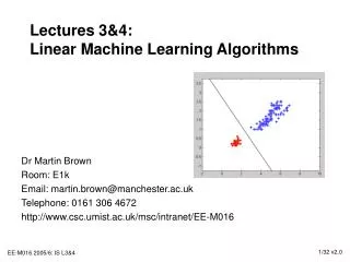
1. Lectures on Machine Learning Tommaso Dorigo, INFN-Padova Braga, March 25-27, 2019

2. Two words about your lecturer I work for INFN – Istituto Nazionale di Fisica Nucleare, in Padova Am a member of the CMS collaboration at CERN (2001-) • formerly (1992-2012) also a member of CDF @ Tevatron Long-time interest in statistics; member of CMS Statistics Committee, 2009-, and chair, 2012-2015 Developed several MVA algorithms for data analysis in HEP (Hyperball, MuScleFit, Inverse bagging, Hemisphere mixing, INFERNO) Editor of Reviews in Physics, an Elsevier journal Scientific coordinator of AMVA4NewPhysics, ITN network on MVA for HEP Scientific coordinator of accelerator-based research for INFN-Padova Blogging about physics since 2005 - www.science20.com , formerly at http://dorigo.wordpress.com and http://qd.typepad.com/6/ In 2016 I wrote a book on searches for signals in CDF  When I don't do physics or statistics I play chess / piano

3. Notes on my lectures • My slides are full of text! • this makes it harder to focus on what I actually say during the lecture... • On the other hand, they offer clarity for offline consumption / consultation Try to pay attention to me rather than on the projected text. You will probably get the gist of it sooner. • I have way too much material the subject is vast! We will have to skip some things / go fast here and there • I am here at your service • Some of the things we will go over are highly non-intuitive, so I expect you to be confused if you have no previous understanding of a topic. • hence please ask questions if you do not understand something. You need not raise your hand. • sometimes I may omit answering straight away / the question may be better covered in later material • I will be at your service also after the school • please email me at tommaso.dorigo@gmail.com if you have nasty questions on the topics covered during the lectures, and I will do my best to answer them.

4. Suggested reading These lectures are based on a number of different sources, as well as on some personal alchemy I tried to provide references but sometimes I failed [apologies...] A formal treatment of most of the covered material, and more in-depth than what I can go here, is offered in a couple of excellent textbooks: Hastie, Tibshirani, Friedman: The elements of statistical learning  AVAILABLE ONLINE FOR FREE! Narsky, Porter: Statistical Analysis techniques in Particle Physics, Wiley

5. Other credits Besides the textbooks quoted above, the production of these lectures also benefited from perusing additional assorted material: • Trevor Hastie's lectures on Statistical Learning, Padova 2017 • Some material from Michael Kagan's lectures at TASI 2017 • One or two ideas from Ilya Narsky's lectures on ML with MatLab, 2018 • A couple of graphs from Lorenzo Moneta's lecture at last year's school • Some slides from interesting presentations at ACAT 2019 Plus random plots / stuff I collected around

6. Contents - 1 Lecture 1: An introduction to Machine Learning • Introduction • Map of ML problems • Supervised and unsupervised learning • Density estimation • kNN • Divergence measures • Resampling techniques • The data • The model

7. Contents - 2 Lecture 2: Classification and decision trees • Classification • Loss minimization • A couple of methods • Fisher linear discriminants • Support vector machines • Decision trees • random forests • boosting techniques

8. Contents - 3 Lecture 3: NNs and HEP applications • Neural networks • Playing with NNs • Advanced techniques • INFERNO • DNNs • Convolutional NNs • Genetic algorithms • Practical tips • Machine Learning in HEP • Generalities • kNN for Hbb • Clustering for HH theory space benchmarking • Higgs Kaggle challenge • Conclusions

9. Lecture 1An introduction to Machine Learning

10. INTRODUCTION

11. Machine Learning is all around us

12. Areas of development for ML tools More market-driven: • Speech and handwriting recognition • often the previous step to NLP • Search engines, advertising • ways to guess what you want • Stock market analysis, predictive models, fraud detection More research-oriented: • Master closed systems (go, chess, computer games) • Natural language processing • allows computers to understand, interpret and manipulate human language • Self-driving cars, object and image recognition, robotics • methods to give spatial awareness to machines • AGI • Distinction more and more blurred as applications pop up • For fundamental physics, both areas offer cues

13. The path to Artificial Intelligence • Alan Turing: machine shuffling 0's and 1's can simulate any mathematical deduction or computation • the Chinese room • Dartmouth conference, 1956  many astonishing developments, checkers, automated theorem solvers • and funding from US defense budget • In the seventies, research effort dampened • Eighties: Expert systems • Nineties: the second AI winter • Solutions to closed system problems; deep blue  alpha zero • Development of Neural Networks • Toward AGI

14. Is AI desirable? Humanity is going to face in the next few decades the biggest "growing pain" of its history: how to deal with the explosive force of artificial intelligence Once we create a superintelligence, there is no turning back – in terms of safeguards we have to "get it right the first time", or we risk to become extinct in a very short time But we cannot stop AI research, no more than we could stop nuclear weapons proliferation Interesting times ahead!

15. Can we define Machine Learning? No self-respected lecture on Machine Learning avoids defining ML at the very beginning, and who am I to blow against the wind? There are various options on how to define ML. Things I have heard around: • “[Machine Learning is the] field of study that gives computers the ability to learn without being explicitly programmed.” - Arthur Samuel (1959) • ok, but learning what? • Wikipedia: "A scientific discipline concerned with the design and development of algorithms that allow computers to evolve behaviors based on empirical data" • correct but slightly vague • Mitchell (1997) provides a succinct definition: “A computer program is said to learn from experience E with respect to some class of tasks T and performance measure P , if its performance at tasks in T , as measured by P , improves with experience E" • The fitting of data with complex functions • in the case of ML, we learn the parameters AND the function • Mathematical models learnt from data that characterize the patterns, regularities, and relationships amongst variables in the system • more lengthy description of "fitting data"

16. Can we agree on what "Learning" is? Maybe this really is the relevant question. Not idle to answer it, as by clarifying what our goal is we take a step in the right direction Some definitions of Learning: • the process of acquiring new, or modifying existing, knowledge, behaviors, skills, values, or preferences • the acquisition of knowledge or skills through study, experience, or being taught. • becoming aware of (something) by information or from observation. • Also, still valid is Mitchell's definition in previous slide In general: learning involves adapting our response to stimuli via a continuous inference. The inference is done by comparing new data to data already processed. How is that done? By the use of analogy.

17. What about analogies? Analogies: arguably the building blocks of our learning process. We learn new features in a unknown object by analogy to known features in similar known objects This is true for language, tools, complex systems – EVERYTHING WE INTERACT WITH ... But before we even start to use analogy for inference or guesswork, we have to classify unknown elements in their equivalence class! (Also, one has to define a metric along which analogous objects align) In a sense, Classification is even more "fundamental" in our learning process than is Analogy. Or maybe we should say that classification is the key ingredient in building analogies.

18. Classification and the scientific method Countless examples may be made of how breakthroughs in the understanding of the world were brought by classifying observations • Mendeleev's table, 1869 (150 years ago!) • Galaxies: Edwin Hubble, 1926 • Evolution of species: Darwin, 1859 (classification of organisms was instrumental in allowing a model of the evolution, although he used genealogy criteria rather than similarity) • Hadrons: Gell-Mann and Zweig, 1964

19. Classification is at the heart of Decision Making • Finding similarities and distinctions between elements, creating classes, looks like • an abstract task • Yet it is at the heart of our decision making process • in a game, choosing the next move entails a classification of the possible actions as • good or bad ones, as a preprocessing step before going "deep" in the analysis • an expert system driving your vehicle must constantly decide how to react to external • stimuli: it does so by classifying them (potentially dangerous  requires choice of proper • reaction; irrelevant  can be ignored) • Decisions are informed by previous experience, and by information processing • That is how we "comprehend" the world and assign it to some description • Ultimately, an important component of intelligence is the continuous processing of our • sensorial inputs, classifying them to react one way or the other to them

20. Classes of Statistical Learning algorithms Supervised: if we know the probability density of S and B, or if at least we can estimate it  E.g. we use "labeled" training events ("Signal" or "Background") to estimate p(x|S), p(x|B) or their ratio Semi-supervised: it has been shown that even knowing the label for part of the data is sufficient to construct a classifier Un-supervised: if we lack an a-priori notion of the structure of the data, and we let an algorithm discover it without e.g. labeling classes  cluster analysis, anomaly detection, unconditional density estimation. We may also single out: Reinforcement learning: the algorithm learns from the success or failure of its own actions  E.g. a robot reaches its goal or fails

21. A map to clarify the players role Machine Learning Unsupervised learning Develop model to group and interpret data without labels Semi-supervised Learning Data only partly labeled Supervised learning Develop predictive model based on labelled data anomaly detection find outliers Regression The output is continuous Clustering Learn ways to partition the data Density Estimation Find p(x) Classification The output is nominal, categorical, unordered / ordered

22. A more complete list of ML tasks /1 Classification and Regression are important tasks belonging to the "supervised" realm. But there are many other tasks: • Density estimation: this is usually an ingredient of classification, but can be a task of its own. • Clustering: find structures in the data, organize by similarity. Often can be a useful input to other tasks • Anomaly detection (e.g. fraud detection, from the modeling of purchasing habits; or new physics searches!) • Classification with missing inputs: if taken with brute force, this differs from simple classification because one is looking for a set of functions, each mapping into the categorical output a vector x with a different set of missing components (but: better to use a probabilistic model to handle it)

23. A more complete list of ML tasks /2 • Structured output: • Transcription: e.g. transform unstructured representation of data into discrete textual form; e.g. images of handwriting or numbers (Google Street view does it with DNN for street addresses), or speech recognition from audio stream • Machine translation • parsing sentences into grammatical structures • image segmentation, e.g. aerial pictures  road positions or land usage • image captioning • Synthesis, sampling: e.g. speech synthesis (structured output with no single correct output for each input); GANs can be used for e.g. generating artificial data • Missing values inputation: this can be a very complex task – Netflix ran a challenge on it to understand customer preferences • Denoising: obtain the clean example from a corrupt one x*, get p(x|x*)

24. The supervised learning problem • Starting point: • A vector of n predictor measurements X (a.k.a. inputs, regressors, covariates, features, independent variables). • One has training data {(x,y)}: events (or examples, instances, observations...) • The outcome measurement Y (a.k.a. dependent variable, or response, or target) • In classification problems Y can take a discrete, unordered set of values (signal/background, index, type of class) • In regression, Y has a continuous value • Objective: • Using the data at hand, we want to predict y* given x*, when (x*,y*) does not necessarily belong to the training set. • The prediction should be accurate: |f(x*)-y*| must be small according to some useful metric (se later) • We would like to also: • understand what feature of X affects the outcome and how • assess the quality of our prediction

25. Example: the Netflix challenge

26. The unsupervised learning problem • Starting point: • A vector of n predictor measurements X (a.k.a. inputs, regressors, covariates, features, independent variables). • One has training data {x}: events (or examples, instances, observations...) • There is no outcome variable Y • Objective is much fuzzier: • Using the data at hand, find groups of events that behave similarly, find features that behave similarly, find linear combinations of features exhibiting largest variation • Hard to find a metric to see how well you are doing • Result can be useful as a pre-processing step for supervised learning

27. Ideal predictions, a' la Bayes For a regression problem, the best prediction we can make for Y based on the input X=x is given by the function f(x) = Ave (Y|X=x) This is the conditional expectation: you just derive the Y average for all examples having the relevant x. • It is the best predictor if we want to minimize the average squared error, Ave (Y-f(X))2. • But it is NOT the best predictor if you use other metrics. E.g., if you wish to minimize Ave |Y-f(X)| you should rather pick... Who can guess it? f(x) = Median (Y|X=x) If we instead are after a qualitative output Y in {1...M} (a discrete one, as in multi-class classification tasks) what we can do is to compute P (Y=m|X=x) for each m: conditional probability of class m at position X=x; then we take as the class prediction C(x) = Arg maxj {P(Y=j|X=x)}. The above is the majority vote classifier. Problem solved? Let us try and see how to implement these ideas.

28. Implementation To predict Y at X=x*, collect all pairs (x*,y) in your training data, then • For regression, get f(x*) = Ave (y|X=x*) • For classification, get c(x*) = Arg maxj {P(Y=j|X=x*)} Alas, this would be good, but... We usually have sparse training data, obtained by forward simulation. Our simulator gives p(x|y) but the process is stochastic. That means we cannot invert the simulator, extracting p(y|x)! In most cases we have NO observations with X=x*. Who you're gonna call ? Density estimation methods!

29. DENSITY ESTIMATION

30. Density Estimation Given a sample of data X, one wishes to determine their prior PDF p(X). One can solve this with parametric or non-parametric approaches. Parametric: find a model within a class, which fits the observed density  an assumption is necessary as the starting point Non-parametric: sample-based estimators. The most common is the histogram. NP density estimators have a number of attractive properties for experimental sciences: • are easy to use for two things dear to HEP/astro-HEP: efficiency estimates (e.g. from Bernoulli trials) and for background subtraction • lend themselves to be good inputs to unfolding methods • are an excellent visualization tool, both in 1 and 2D S+B B S

31. The empirical density estimate With sparse data, the most obvious estimate of the density from which i.i.d. data {xi} are drawn is called "empirical probability density function" (EPDF), which can be obtained by placing a Dirac delta function at each observation xi: Of course, the EPDF is rarely useful in practice as a computation tool. However, it is a common way of visualizing 2D or 3D data (scatterplots)

32. Histograms Histograms are a versatile, intuitive, ubiquitous way to get a quick density estimate from data points: h(x) = Sumi=1...N I(x-xi;w) where w is the width of the bin, and I is a uniform interval function (indicator function), I(x;w) = 1 for x in [-w/2,w/2], = 0 otherwise The density estimate provided by h(x) is then f(x) = h(x)/(Nw) Yet histograms have drawbacks: • they are discontinuous • they lose information on the true location of each data points through the use of a "regularization", the bin width w • not unique: there is a 2D infinity of histogram-based PDF estimates possible for each dataset, depending on binning and offset. I(x;w) w x xi

33. Kernel density estimation A useful generalization of the histogram is obtained by substituting the indicator function with a suitable "kernel": The kernel function k(x,w) is normalized to unity. It is typically of the form The advantage of using a kernel instead than a delta is evident: we obtain a continuous, smooth function. This comes, of course, at the cost of a modeling assumption. A common kernel is the Gaussian distribution; the results however depend more on the smoothing parameter w than on the choice of the specific form of k. The "kernelization" of the data can be operated in multiple dimensions too. The kernels operating in each component are identical but may have different smoothing parameters: A different extension of the KDE idea is to adapt the smoothness parameter w to reflect the precision of the local estimate of the data density  adaptive kernel estimation

34. Ideograms A further extension of KDE is the use of different kernels for different data points ideograms. This may be very useful if the data coordinate x comes endowed with information on its measurement precision σ. In that case we may substitute the point with a Gaussian kernel, whose smoothing parameter w is equal to the precision σ. This improves the overall density estimate The ideogram method is sometimes used in HEP, e.g. it has been employed in top quark mass measurements. The PDG uses it to report the PDF of a unknown parameter when the individual estimates carry different uncertainty AND there is tension between the estimates (such that the weighted average is not necessarily the whole story)

35. Going multi-D: K-Nearest Neighbours • The kNN algorithm tries to determine the local density • of multi-dimensional data by finding how many data points • are contained in the surroundings of every point in feature space • One usually "weighs" data points with a suitable • function of the distance from the test point • Problem: how to define the distance in an abstract space? • Also, your features might include real numbers, categories, days of the week, etcetera... • In general, it is useful to remove the dimensional nature of the features • General recipe: standardization • - for continuous variable x: find variance σ2, obtain standardized variable y2 = x2 /σ2 • for categorical variable c: • if target has large variance along c, can keep it as is (defines hyperplane, will only • use data with c*=c to estimate local density) • otherwise may still try to standardize

36. More on kNN Once the data is properly standardized one can construct an Euclidean distance: kNN density estimates can be endowed with several parameters to improve their performance Most obvious is k: how many events in the ball? Rule of thumb: estimating a mean  if target varies a lot, can use small k; if variation small, k needs to allow precise estimate Common to have k=20-50, but it of course depends on dimensionality D and size N of training data

37. kNN, continued Also crucial to assess: • relative importance of variables: assign larger weight to more meaningful components in the feature space (ones along which target has largest variance) • local gradients-aware: one may try and adapt the shape of the "hyperellipsoid" to reflect how much target y(x) is variable in each direction, at test point x* In general, kNN estimates suffer from a couple of shortcomings: • The evaluation of local density requires to use all data for each point of feature space  CPU expensive (but there are shortcuts) • The curse of dimensionality: for D>8-9, they become insensitive to local density (see next slide)

38. One example In 2003 the Tevatron experiments assessed their chances to observe the Higgs with more data / improved detectors One of the crucial issues: Mbb regression Customized kNN algorithm with balls shaped by local gradient ("Hyperball algorithm") brought down relative mass resolution from 17% to 10%  large increase in observability

39. The Curse of Dimensionality The estimate of density in a D-dimensional space is usually impossible, due to the lack of sufficient labeled data for the calculation to be meaningful. An adequateamount of data must grow exponentially with D for a good representation For high problem dimensionality, the k "closest" events are in no way close to the point where an estimate of the density is sought: This makes kNN impractical for D > 8-10 dimensions In 10 dimensions, if a hypersphere captures 1% of the feature space, it has a radius of 63% in each variable span HEP analyses often have >10 important variables so the kNN has limited use as a generative algorithm for S/B discrimination But, one can apply dimensional reduction techniques to still use it, or resample subspaces

40. What If We Ignore Correlations? All PDF-estimation methods similarly fail when D is large. A "Naïve Bayesian" approach consists in ignoring altogether the correlations between the variables of the feature space That is, one only looks at the "marginals": P is a product of "marginal PDFs" Pi One usually models the Pi with a smoothing of histograms The P(x) thus obtained can be used to construct a discriminant (a likelihood ratio), or more simply, to assign the class label to the highest p(x) given x The method works if correlations are unimportant. In HEP, however, this is not usually the case!

41. A small diversion: parametric density estimators Given an empirical density estimate p(x) obtained by N i.i.d. data points {xi}, we might want/need to formulate our problem as that of finding parameters of a function q(θ) such that it gets "closer" to p(x). The focus is what "closer" means! The density estimation problem can be summarized formally as follows: What we need is to construct a probability divergence D(Q; P) between two smooth probability densities Q:RdR+ and P:RdR+, where Q is defined by a parametric generative model with parameters θ,and P is a target density. If H is a space of densities (), we can define a probability divergence D(P;Q) as a map D:H2R+that enjoys some properties (next slide) The goal is to have a consistent interpretation of D(Q; P) as well as use it to modify the parameters so that Q approaches P.

42. Divergence measures In general, one could argue that all we need is to find some D which guarantees • D(Q,P) = 0  Q=P • D(Q,P) >= 0 There are additional properties we might want D to have; e.g., be a metric. A metric also has the properties that • D(Q,P) = D(P,Q) • D(A,C) < D(A,B) + D(B,C) (triangle inequality) The improved interpretability of distance between densities that is offered by these added properties is an important property. But we might rather prefer our divergence to have other properties. In particular, we wish to make our D a measure of relative information. This is what makes the Kullbach-Leibler divergence KL so useful.

43. The Kullback-Leibler divergence The KL divergence has its origins in information theory, where one wishes to quantify the amount of information contained in data. One defines Entropy Hfor a probability distribution as In base 2, H is the minimum number of bits that encode the available information of p. If we know this, we have a way to quantify the information in our data. Given that, we can extract the information loss we incur in, if we substitute the data p with a model q of it. This is given by the KL divergence, defined as (for discrete datasets)

44. KL / continued What the KL divergence provides is the expectation of the log difference between the probability of data in the original distribution with the approximating distribution. So we could write it as The value of DKL gives us a measure of the number of bits we lose if we approximate p with q. As such, it does not possess one of the properties of a true metric, as DKL(p;q) != DKL(q;p). But its importance cannot be underestimated in ML, as it provides exactly what we need in our attempts to estimate densities by successive approximations.  often used in the definition of loss functions Another way to see DKL: expected number of bits that we have to transmit to a receiver in order to communicate the density Q given that the receiver already knows the density P

45. Example: comparison of divergences The minimization of different divergence measures for a Gaussian model of the data provides quite different answers  This shows that it is important to know what we are using in our minimization problem! Below are some formulations of different choices for probability divergence measures; p is the data and q is the model

46. RESAMPLING TECHNIQUES

47. Resampling Techniques Resampling techniques are pivotal for a number of ML tasks: • hypothesis testing (construction of discriminative methods) • estimation of bias and variance (optimization of predictors) • cross-validation (estimate accuracy of predictors) Resampling allows you to avoid modeling assumptions, as you construct a non-parametric model from the data themselves. The benefits can be huge (as measured e.g. by performance of boosting methods) Here we only briefly flash the generalities of three basic ingredients: • permutation tests • bootstrap • jacknife • cross-validation techniques will treat later The theoretical basis for resampling methods lies with their (usually very good) asymptotic properties of consistency and convergence (in probability)

48. Permutation Sampling A x B Permutation sampling is mainly used in hypothesis tests; usually the question is: are datasets A {x1...XNA} and B {x1...xNB} sampled from the same parent PDF? The way to answer is to form a sensitive statistic T (say: the mean of the observations) and compare quantitatively the difference between TA and TB ΔT* = TA-TB with what one would expect if the PDF were the same. x ΔT* ΔT The comparison requires to know how T distributes under the null hypothesis (green curve). Here permutation comes in: we assume A=B, merge A+B=C, and sample the NA+NB observations creating all possible pairs of splits A', B' still of size {NA,NB}, computing distances ΔT=TA'-TB'. This provides all the information in the data about the distribution of ΔT. The permutation test makes no model assumptions, so it is called an exact test.

49. The Bootstrap The Bootstrap (B.Efron, 1979) is called this way because it allows to "pull oneself up from one's own bootstraps". Motivating problem: get the variance of an estimator of a parameter θ,for a sample of i.i.d. observations {x1...xN}. We may generate M replicas of the dataset X by repeatedly picking N observations at random from X, with replacement. Then we estimate θ in each replica, and proceed to obtain a sample mean and variance with the , You get an estimate of variance without assumptions of the distribution

50. Bootstrap-cum-density estimation example: hhbbbb CMS 2017 In a recent CMS search of hhbbbb production (CMS-PAS-HIG-17-017), the background was dominated by QCD multijet production – notoriously a difficult process to model with MC simulations In order to train a classifier, you need a good multi-D model of the features... A synthetic background sample was constructed by mixing hemispheres The idea is that QCD gives two hard quarks or gluons that scatter off one another, and the complexity arises independently, as a combination of FSR, pileup, MI  can try to create models of single "halves" of the events