The Phillips curve

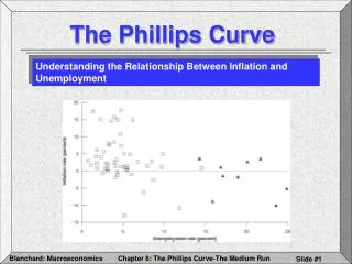
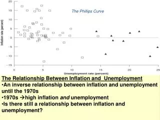
1. The Phillips curve • In last week’s lecture, we brought the labour market equations into the IS-LM framework and derived the aggregate supply-aggregate demand framework. The advantage of AS-AD over IS-LM is that you can use the AS-AD to talk about prices and unemployment. • A.W. Phillips (a NZ raised in Australia) found a negative relation between inflation and unemployment in the United Kingdom on data from the previous century.

2. Phillips curve in Australia 1960s

3. Moving from prices to inflation • Our labour market equations were in price levels, where here we would like to talk in terms of inflation. Can we put our labour market equations in terms of inflation? • Our labour market equilibrium equation: P = Pe (1 + μ )F(u, z) • The we “linearize” F(.) by setting: F (u, z) = 1 – αu + z

4. Moving from prices to inflation • So we get: P = Pe (1 + μ )(1 – αu + z) • This can be rewritten in inflation (π)and expected inflation (πe) as: π = πe + (μ + z) - αu • The derivation is in the appendix for Chapter 8 and is NOT required to know. Simply know that this is only true for “low” levels of inflation.

5. The new labour market equation • Our new labour-market equilibrium condition is: π = πe + (μ + z) - αu • A rise in expected inflation increases current inflation one-for-one. • A rise in unemployment lowers inflation by the amount α. • A rise in the mark-up increases inflation, as do factors, z, that increase the wage-setting term, F(u, z).

6. Policy implications • If this new relation between inflation and unemployment is true, it means that governments had a tool to control inflation. • If governments were willing to raise inflation, they would achieve a lower level of unemployment. • Governments could permanently drive unemployment below the “natural rate of unemployment” by permanently raising inflation.

7. Policy implications • There is an “inflation-unemployment trade-off”. Governments could “choose” an optimal inflation-unemployment mix along the Phillips curve that best suited them. • Labor governments might choose a trade-off with lower unemployment. Liberal governments might choose a trade-off with lower inflation.

8. Phillips curve break-down 1977 1983 1993 1970 2003

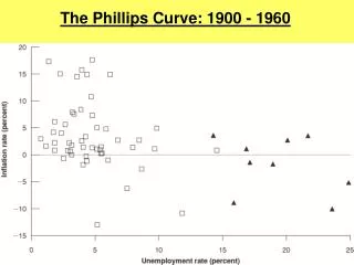
9. What caused the breakdown? • The governments assumed that the expected inflation rate, πe, didn’t change. • But the Phillips curve relationship: π = πe + (μ + z) - αu • The y-intercept is πe + (μ + z) and the slope is – α. So any change in πe shifts the Phillips curve relation out. • Governments in the 1970s assumed that the Phillips curve didn’t move. They were obviously wrong.

10. Inflation expectations • So the Phillips curve depends crucially on how people form expectations of inflation. • Let’s say that inflationary expectations are slow to adjust, so: πte = θπt-1 • The we can make this substitution into the Phillips curve equation: πt = θπt-1 + (μ + z) - αut

11. Expectations πt = θπt-1 + (μ + z) - αut • For θ = 0, we have a Phillips curve that does not move. For θ = 1, we have the relation: πt - πt-1 = (μ + z) - αut • So the change in inflation depends on the unemployment rate. • We can also represent this equation in terms of the natural rate of unemployment.

12. Natural rate of unemployment • If inflation is equal to expected inflation, we are at our “natural rate”, so we have: π = πe + (μ + z) - αun • But π = πe, so we can simplify to: 0 = (μ + z) - αun α un = (μ + z) or un = (μ + z) / α • Our natural rate of unemployment is: • Higher the higher is the firm mark-up; and • Lower the greater is the reaction of wage increases to unemployment, α.

13. Natural rate of unemployment • Substituting into our Phillips curve relation for θ = 1, we get: πt - πt-1 = αun - αut = - α (ut – un) • So if unemployment is lower than the natural rate, inflation will increase by α. • The way to lower inflation is to have unemployment higher than the natural rate. • The only way to keep inflation steady is to have unemployment equal to the natural rate- the non-accelerating rate of unemployment (NAIRU).

14. Policy implications • There is no permanent trade-off between inflation and unemployment, as governments assumed in the 1960s and 1970s. • If the government tries to push unemployment permanently below the natural rate, it will have permanently rising inflation rates. • This is what happened to governments in the 1970s. The Phillips curve kept shifting as inflationary expectations rose.