Download
1 / 35
350 likes | 469 Views
Economic Analysis for Business Session XVI: Theory of Consumer Choice – 2 (Utility Analysis) with Production Function. Instructor Sandeep Basnyat 9841892281 Sandeep_basnyat@yahoo.com. Utility Function. Two ways to represent consumer preferences: Indifference Curve Utility

E N D
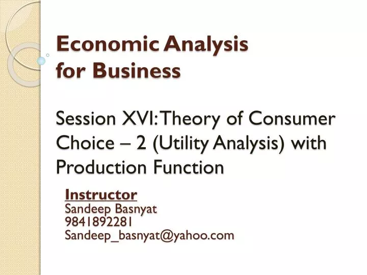
Economic Analysis for BusinessSession XVI: Theory of Consumer Choice – 2 (Utility Analysis) with Production Function InstructorSandeep Basnyat 9841892281 Sandeep_basnyat@yahoo.com
Utility Function • Two ways to represent consumer preferences: • Indifference Curve • Utility • Utility is an abstract measure of the satisfaction that a consumer receives from a bundle of goods. • Indifference Curve and Utility are closely related. • Because the consumer prefers points on higher indifference curves, bundles of goods on higher indifference curves provide higher utility.
Cones/ Hour Total Utility (Utility/Hr) 150 0 0 120 1 50 Total Utility in Utils 2 90 50 3 120 4 140 0 0 1 2 3 4 5 5 6 150 140 Cones per hour 0 Utility Function (Similar to Production Function) 140 6
∆Tot. Utility ∆Consumption 0 Marginal Utility • The marginal utilityof consumption of any input is the increase in utility arising from an additional unit of consumption of that input, holding all other inputs constant. • Marginal Utility =
Cones/ Hour Total Utility (Utility/Hr) 0 0 1 50 2 90 3 120 4 140 5 6 150 140 0 Marginal Utility Marginal Utility (Utility/Cone) The Law of Diminishing Marginal Utility The tendency for the additional utility gained from consuming an additional unit of a good to diminish as consumption increases beyond some point 50 40 30 20 10 -10
0 Utility Maximization Assume: • Two goods: Chocolate and vanilla ice cream • Price of chocolate = $2/pint • Marginal Utility from chocolate = 16 utils/pint • Price of vanilla = $1/pint • Marginal Utility from vanilla = 12 utils/pint • Sarah’s ice cream budget = $400/yr • Currently Sarah’s consumption of: Vanilla ice-cream = 200 pints chocolate ice cream = 100 pints Is Sarah maximizing her total utility? If not, should she buy more chocolate and less vanilla or more vanilla and less chocolate?
0 Utility Maximization Here, Marginal Utility from chocolate = 16 utils/pint Price of chocolate = $2/pint Marginal utility from chocolate/$ = 16/2 = 8 utils/$ For every $ Sarah spends on chocolate, she derives additional utlity of 8 . Similarly, • Marginal Utility from vanilla = 12 utils/pint • Price of vanilla = $1/pint • Marginal utility from chocolate/$ = 12/1 = 12 util/$ For every $ Sarah spends on vanilla, she derives additional utlity of 12 Sarah should spend more on vanilla than chocolate. By How much?
0 Utility Maximization The Rational Spending Rule: Spending should be allocated across goods so that the marginal utility per dollar is the same for each good. i.e, ,Marginal utility from chocolate/$ = Marginal utility from vanilla / $ From our example, Marginal utility from chocolate/$ (= 16/2 = 8 utils/$) = Marginal Utility from chocolate / Price of chocolate = MUc / Pc Similarly, Marginal utility from vanilla/$ (= 12/1 = 12 util/$) = Marginal Utility from vanilla / Price of vanilla = MUv / Pv The Rational Spending Rule: MUc / Pc = MUv / Pv
0 Utility Maximization The Rational Spending Rule: Spending should be allocated across goods so that the marginal utility per dollar is the same for each MUc / Pc = MUv / Pv or, MUc / MUv = Pc / Pv or, MUv / MUc = Pv / Pc or MUx / MUy = Px / Py Here, MUv / MUc = Marginal Rate of substitution of vanilla for chocolate Pv / Pc = Relative price of vanilla and chocolate Therefore, How much should Sarah spend on each? MRS = MUv / Muc = Pv / Pc
0 Utility Maximization At present, MRS = MUv / Muc = 12 /16 = 0.75 and, Pv / Pc = 1/2 = 0.5 So, Sarah’s should reschedule her spending such that her MRS = 1/2.
0 Utility Maximization-Change in Prices • Assume • Budget = $400 • MUc = 20; MUv = 10 • PC = $2 & PV = $1 • QC = 75 & QV = 250 So, MUc / Pc = 20 / 2 = 10 MUv / Pv = 10 / 1 = 10 = MUc / Pc If the price of chocolate falls to $1. Should you buy more chocolate or less?
0 Utility Maximization-Change in Prices • Assume • Budget = $400 • MUc = 20; MUv = 10 • PC = $2 & PV = $1 • QC = 75 & QV = 250 So, MUc / Pc = 20 / 2 = 10 MUv / Pv = 10 / 1 = 10 = MUc / Pc If the price of chocolate falls to $1. Should you buy more chocolate or less? Now, MUc / Pc = 20 / 1 = 20. Should buy more chocolate.
Worked out examples Jane receives utility from days spent traveling on vacation domestically (D) and days spent traveling on vacation in a foreign country (F), as given by the utility function U(D,F) = 10DF. In addition, the price of a day spent traveling domestically is $100, the price of a day spent traveling in a foreign country is $400, and Jane’s annual travel budget is $4,000. • Find Jane’s utility maximizing choice of days spent traveling domestically and days spent in a foreign country. • Find her total utility. Hint: • Find consumer’s optimum using the rational spending rule. • Marginal utility of D or F can be found by differentiating Total Utility keeping one factor constant at a time.
Worked out examples Solution: The optimal bundle is where the slope of the indifference curve (MRS) is equal to the slope of the budget line (Relative price of the good), and Jane is spending her entire income. So: PD / PF = 100/400 = 1/4 MRS = MUD / MUF = F. 10D1-1/D. 10F1-1 = 10F/10D = F/D Setting the two equal we get: F / D = 1/4 or, 4F = D ---(i) From the above question: 100 D + 400 F = 4000 -------(ii) Solving the above two equations gives D=20 and F=5. Utility is 1000.
L(no. of workers) Q(bushels of wheat) 3,000 2,500 0 0 2,000 1 1000 1,500 Quantity of output 2 1800 1,000 3 2400 500 4 2800 0 0 1 2 3 4 5 5 3000 No. of workers 0 Recall Example: Production Function • Relationship between input and output
∆Q ∆Q ∆L ∆K Recall: Properties of Production Functions: Returns to Scale production functions have increasing, constant or decreasing returns to scale. (i) Q = 3L (ii) Q = L0.5 (iii) Q = L2 (Constant) (Decreasing) (Increasing) Marginal product of labor (MPL) = Marginal product of capital (MPk) =
Total Product • Total Product of Labour: Maximum output (Q) produced by the labour keeping the capital constant. Total Product of Labour function: Q = TPL = f (K, L) • Total Product of Capital: Maximum output (Q) produced by the capital keeping the labour constant. Total Product of capital function: Q = TPK = f (K, L) • Average Product of Labour (APL) = TPL / L • Average Product of Capital (APK) = TPK / K
Worked out examples • For the Production function: Q = 10K0.5L0.5 whose labour input (L) is 4, capital (K) is fixed 9 units calculate: TPL and APL Solution: • (TPL) = Q = f (K, L) = 10K0.5L0.5 = 10 x 90.5 x 40.5 = 10 x 3 x 2 = 60 • APL = TPL / L = 60 / 4 = 15
Relationship between Total, Average, & Marginal Products: Assume K is fixed and L is variable -- -- 52 52 60 56 58 56.7 50 55 38 51.6 28 47.7 18 43.4 10 39.3 4 35.3 -4 31.4
Total, Average & Marginal Products -- -- 52 52 56 60 56.7 58 55 50 51.6 38 47.7 28 43.4 18 39.3 10 35.3 4 31.4 -4
Q2 Q1 Total product Q0 L0 L1 L2 Average product L0 L1 L2 Marginal product Total, Average & Marginal Product Curves Stage 1 Stage 2 Stage 3 Panel A Increasing Marginal returns Diminishing Marginal returns Panel B Negative Marginal returns
Marginal Product functions If the Production Function is Cobb-Douglas: Q = AKαLβ Then, • Marginal Product of Labour (MPL) = dQ / dL = βAKαLβ-1 (keeping K constant) • Marginal Product of Capital (MPK) = dQ / dK = αAKα-1Lβ (keeping L constant) • Value of Marginal Product of Labour (VMPL) = P x MPL
Worked out examples • For the Production function: Q = 10K0.5L0.5 whose labour input (L) is 4, selling price per unit is Rs. 5, capital (K) is fixed 9 units calculate: MPL, VMPL. Solution: • MPL = dQ / dL = βAKαLβ-1 = 10 (1/2)K0.5L0.5-1 =5(K0.5 / L0.5) = 5 x (3/2) = 7.5 • VMPL = P * MPL = 5 x 7.5 = Rs. 37.5
How many Labour or Capital to hire? What determines how many extra labour is hired? Suppose, MPL = 2 units; Price of each unit sold = $20,000 Cost of hiring worker (wage rate) = $30000 Will the firm hire the worker? Additional Revenue for the firm from hiring extra labour (Marginal Revenue Product : MRPL) = 2 x 20,000 = $40,000 Additional cost for the firm for hiring extra worker (Wage Rate -W) = $30,000 Formally, Firms hires extra worker until, MRPL = P. MPL = w (Note: In Perfectly competitive market, P = MR. So, MRPL = MR. MPL • Similarly, the in case of capital, capital could be employed until MRPK equals the price of the capital (r): MRPK = r
Worked out example For the Production function: Q = 10K0.5L0.5 whose, capital (K) is fixed 9 units, selling price per unit is Rs. 5 and wage rate is Rs. 3, calculate how many labour should be hired. Find out the profit maximizing rate of labour hired if the wage rate increased to Rs.5.
Worked out example For the Production function: Q = 10K0.5L0.5 whose, capital (K) is fixed 9 units, selling price per unit is Rs. 5 and wage rate is Rs. 3, calculate how many labour should be hired. Find out the profit maximizing rate of labour hired if the wage rate increased to Rs.5. Solution: MRPL = P. MPL = P. dQ / dL = P. βAKαLβ-1 = 5.10 (1/2)K0.5L0.5-1 =25(K0.5 / L0.5) = 25 x (3/L) = 75/ L0.5 Total labour hired until: MRPL = w 75/ L0.5 = 3 L = 252 = 625 Therefore total no. of labour hired is 625. If w = 5, then profit maximizing no. of labour hired is: 75/ L0.5 = 5. Therefore, L = 225
Production Isoquants • In the long run, all inputs are variable & isoquants are used to study production decisions • An isoquant is a curve showing all possible input combinations capable of producing a given level of output • Isoquants are downward sloping; if greater amounts of labor are used, less capital is required to produce a given output
Production Isoquants • Assume a Cobb-Douglas Production function: Q = 100K0.5L0.5 If K = 8 and L = 2, Q = 400 To obtain, Q = 400, other possible options: K = 4 and L = 4 or, K = 2 and L = 8
C B D E A Q1 = 400 Typical Isoquants Units of Capital 8 4 Q3 = 600 2 Q2 = 200 2 4 8 Units of Labour 0
Marginal Rate of Technical Substitution • The MRTS is the slope of an isoquant & measures the rate at which the two inputs can be substituted for one another while maintaining a constant level of output
Marginal Rate of Technical Substitution • The MRTS can also be expressed as the ratio of two marginal products:
The Production Isocost • If, No. of capital = K • Per unit price of capital = r • No. of Labour = L • Per unit wage rate = w • Total expenditure on capital and Labour: C = rK + wL • Now, if r= 3 and w = 2, then • Combination of 10 units of capital and 5 units of labour will cost 40. I.e, 40 = 3(10) + 2(5). • There might be others combinations which will result the constant expenditure.
• Isocost Curves The ration w/r is the rate at which K can be traded for L. The ration r/w is the rate at which L can be traded for K. C = rK + wL or •
Profit Maximization As stated before, • Firms will hire extra labour and capital until: MRPL = w and MRPK = r PxMPL = w and PxMPK = r Dividing, MPL / MPK = w / r MPL / w = MPK / r ……………..(i) Equation (i) is known as efficiency condition. Or Least cost combination input. Meaning: if a firm is maximizing in the above condition, then it is efficiently operating.