Download
1 / 21
210 likes | 336 Views
This paper explores max weight learning algorithms to tackle scheduling problems in environments with unknown parameters. The focus is on a two-stage decision-making framework where a primary decision reveals a random vector, which influences subsequent decisions affecting queue dynamics and incurs penalty vectors. The research presents motivating examples including min power scheduling and diversity backpressure routing, highlighting innovative approaches that do not require prior knowledge of channel state distributions. The methods leverage stochastic Lyapunov optimization techniques to minimize average penalties effectively while ensuring system stability.

E N D
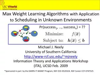
Max Weight Learning Algorithms with Application to Scheduling in Unknown Environments Pr(success1, …, successn) = ?? Michael J. Neely University of Southern California http://www-rcf.usc.edu/~mjneely Information Theory and Applications Workshop (ITA), UCSD Feb. 2009 *Sponsored in part by the DARPA IT-MANET Program, NSF OCE-0520324, NSF Career CCF-0747525
5 6 0 1 2 3 4 • Slotted System, slots t in {0, 1, 2, …} • Network Queues: Q(t) = (Q1(t), …, QL(t)) • 2-Stage Control Decision Every slot t: • 1) Stage 1 Decision: k(t) in {1, 2, …, K}. • Reveals random vector w(t) (iid given k(t)) • w(t) has unknown distribution Fk(w). • 2) Stage 2 Decision:I(t) in I(a possibly infinite set). • Affects queue rates: • A(k(t), w(t), I(t)) , m(k(t), w(t),I(t)) • Incurs a “Penalty Vector” x(t): • x(t) = x(k(t), w(t), I(t))
Stage 1: k(t) in {1, …, K}. Reveals random w(t). Stage 2: I(t) in I. Incurs Penalties x(k(t), w(t), I(t)). Also affects queue dynamics A(k(t), w(t), I(t)) , m(k(t), w(t),I(t)). Goal: Choose stage 1 and stage 2 decisions over time so that the time average penalties x solve: f(x), hn(x) general convex functions of multi-variables
Motivating Example 1: Min Power Scheduling with Channel Measurement Costs S1(t) A1(t) Minimize Avg. Power Subject to Stability S2(t) A2(t) AL(t) SL(t) If channel states are known every slot: Can Schedule without knowing channel statistics or arrival rates! (EECA --- Neely 2005, 2006) (Georgiadis, Neely, Tassiulas F&T 2006)
Motivating Example 1: Min Power Scheduling with Channel Measurement Costs S1(t) A1(t) Minimize Avg. Power Subject to Stability S2(t) A2(t) AL(t) SL(t) If “cost” to measuring, we make a 2-stage decision: Stage 1: Measure or Not? (reveals channels w(t) ) Stage 2: Transmit over a known channel? a blind channel? -Li and Neely (07) -Gopalan, Caramanis, Shakkottai (07) Existing Solutions require a-priori knowledge of the full joint-channel state distribution! (2L , 1024L ? )
Motivating Example 2: Diversity Backpressure Routing (DIVBAR) 3 2 error 1 [Neely, Urgaonkar 2006, 2008] broadcasting Networking with Lossy channels & Multi-Receiver Diversity: DIVBAR Stage 1: Choose Commodity and Transmit DIVBAR Stage 2: Get Success Feedback, Choose Next hop If there is a single commodity (no stage 1 decision), we do not need success probabilities! If two or more commodities, we need full joint success probability distribution over all neighbors!
Stage 1: k(t) in {1, …, K}. Reveals random w(t). Stage 2: I(t) in I. Incurs Penalties x(k(t), w(t), I(t)). Also affects queue dynamics A(k(t), w(t), I(t)) , m(k(t), w(t),I(t)). Goal: Equivalent to: Where g(t) is an auxiliary vector that is a proxy for x(t).
Stage 1: k(t) in {1, …, K}. Reveals random w(t). Stage 2: I(t) in I. Incurs Penalties x(k(t), w(t), I(t)). Also affects queue dynamics A(k(t), w(t), I(t)) , m(k(t), w(t),I(t)). Equivalent Goal: Technique: Form virtual queues for each constraint. U(t) b h(g(t)) Un(t+1) = max[Un(t) + hn(g(t)) – bn,0] Z(t) x(t) g(t) Zm(t+1) = Zm(t) – gm(t) + xm(t) Possibly negative
Use Stochastic Lyapunov Optimization Technique: [Neely 2003], [Georgiadis, Neely, Tassiulas F&T 2006] Define: Q(t) = All Queues States = [Q(t), Z(t), U(t)] Define: L(Q(t)) = (1/2)[sum of squared queue sizes] Define: D(Q(t)) = E{L(Q(t+1)) – L(Q(t))|Q(t)} Schedule using the modified “Max-Weight” Rule: Every slot t, observe queue states and make a 2-stage decision to minimize the “drift plus penalty”: Minimize:D(Q(t)) + Vf(g(t)) Where V is a constant control parameter that affects Proximity to optimality (and a delay tradeoff).
How to (try to) minimize: Minimize:D(Q(t)) + Vf(g(t)) The proxy variables g(t) appear separably, and their terms can be minimized without knowing system stochastics! Minimize: Subject to: [Zm(t) and Un(t) are known queue backlogs for slot t]
Minimizing the Remaining Terms: Minimize:D(Q(t)) + Vf(g(t))
Solution: Defineg(mw)(t), I(mw)(t) , k(mw)(t) as the ideal max-weight decisions (minimizing the drift expression). Define ek(t): Then: ? k(mw)(t) = argmin{k in {1,.., K}} ek(t) (Stage 1) I(mw)(t) = argmin{I in I} Yk(t)(w(t), I, Q) (Stage 2) g(mw)(t) = solution to the proxy problem
Approximation Theorem: (related to Neely 2003, G-N-T F&T 2006) If actual decisions satisfy: With: (related to slackness of constraints) Then: -All Constraints Satisfied. [B + C + c0V] min[emax – eQ, s – eZ] -Average Queue Sizes < -Penalty Satisfies: f( x ) < f*optimal + O(max[eQ,eZ]) + (B+C)/V
It all hinges on our approximation of ek(t): Declare a “type k exploration event” independently with probability q>0 (small). We must use k(t) = k here. Approach 1: {w1(k)(t), …, wW(k)(t)} = samples over past W type kexplor. events
It all hinges on our approximation of ek(t): Declare a “type k exploration event” independently with probability q>0 (small). We must use k(t) = k here. Approach 2: {w1(k)(t), …, wW(k)(t)} = samples over past W type kexplor. Events {Q1(k)(t), …, QW(k)(t)} = queue backlogs at these sample times.
Analysis (Approach 2): Subtleties: “Inspection Paradox” issue requires use of samples at exploration events, so {w1(k)(t), …, wW(k)(t)} iid. 2) Even so, {w1(k)(t), …, wW(k)(t)} are correlated with queue backlogs at time t, and so we cannot directly apply the Law of Large Numbers!
Analysis (Approach 2): w1(t) w2(t) w3(t) wW(t) tstart t Use a “Delayed Queue” Analysis: Can Apply LLN constant constant
Max-Weight Learning Algorithm (Approach 2): (No knowledge of probability distributions is required!) -Have Random Exploration Events (prob. q). -Choose Stage-1 decision k(t) = argmin{k in {1,.., K}}[ ek(t) ] -Use I(mw)(t) for Stage-2 decision: I(mw)(t) = argmin{I in I} Yk(t)(w(t), I, Q(t)) -Use g(mw)(t) for proxy variables. -Update the virtual queues and the moving averages.
Theorem (Fixed W, V): With window size W we have: -All Constraints Satisfied. [B + C + c0V] min[emax – eQ, s – eZ] -Average Queue Sizes < -Penalty Satisfies: f( x ) < f*q + O(1/sqrt{W}) + (B+C)/V
Concluding Theorem (Variable W, V): Let 0 < b1 < b2 < 1. Define V(t) = (t + 1) b1 , W(t) = (t+1)b2 Then under the Max-Weight Learning Algorithm: -All Constraints are Satisfied. -All Queues are mean rate stable*: -Average Penalty gets exact optimality (subject to random exploration events): *Mean rate stability does not imply finite average congestion and delay. In fact, Average congestion and delay are necessarily infinite when exact optimality is reached. f( x ) = f*q