CS 130 A: Data Structures and Algorithms
CS 130 A: Data Structures and Algorithms. Focus of the course: Data structures and related algorithms Correctness and ( time and space ) complexity Prerequisites CS 20: stacks, queues, lists, binary search trees, … CS 40: functions, recurrence equations, induction, …

CS 130 A: Data Structures and Algorithms
E N D
Presentation Transcript
CS 130 A: Data Structures and Algorithms • Focus of the course: • Data structures and related algorithms • Correctness and (time and space) complexity • Prerequisites • CS 20: stacks, queues, lists, binary search trees, … • CS 40: functions, recurrence equations, induction, … • CS 60:C, C++, and UNIX • Requirements: • Exams: 2 midterms and a final • Homeworks + programming assignments • Programs must run on CSIL machines (Linux) with g++(gcc)
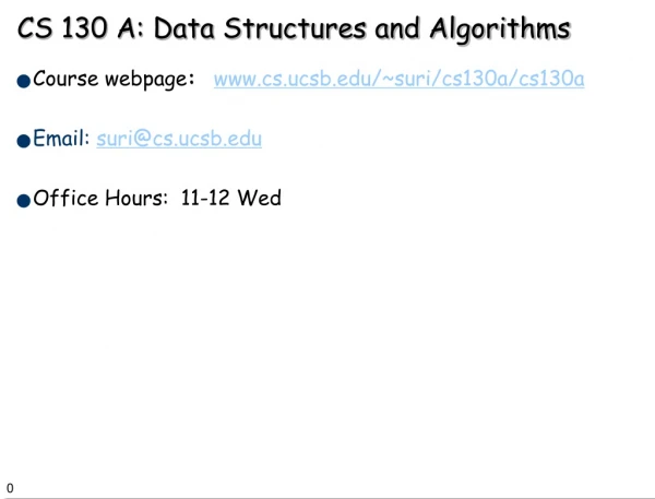
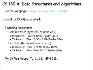
Course Organization • Grading: • Homework: 40%, Midterms: 30%, Final: 30% • Policy: • No late homeworks. • Cheating and plagiaris: F grade and disciplinary actions • Online info:Homepage: www.cs.ucsb.edu/~cs130a • Email:cs130a@cs.ucsb.edu • Teaching assistants: Caijie Zhang (caijie@cs). • One discussion sessions
Introduction • A famous quote: Program = Algorithm + Data Structure. • All of you have programmed; thus have already been exposed to algorithms and data structure. • Perhaps you didn't see them as separate entities; • Perhaps you saw data structures as simple programming constructs (provided by STL--standard template library). • However, data structures are quite distinct from algorithms, and very important in their own right.
Objectives • The main focus of this course is to introduce you to a systematic study of algorithms and data structure. • The two guiding principles of the course are: abstraction and formal analysis. • Abstraction: We focus on topics that are broadly applicable to a variety of problems. • Analysis: We want a formal way to compare two objects (data structures or algorithms). • In particular, we will worry about "always correct"-ness, and worst-case bounds on time and memory (space).
Textbook • Textbook for the course is: • Data Structures and Algorithm Analysis in C++ • by Mark Allen Weiss • But I will use material from other books and research papers, so the ultimate source should be my lectures.
Course Outline • C++ Review (Ch. 1) • Algorithm Analysis (Ch. 2) • Sets with insert/delete/member: Hashing (Ch. 5) • Sets in general: Balanced search trees (Ch. 4 and 12.2) • Sets with priority: Heaps, priority queues (Ch. 6) • Graphs: Shortest-path algorithms (Ch. 9.1 – 9.3.2) • Sets with disjoint union: Union/find trees (Ch. 8.1–8.5) • Graphs: Minimum spanning trees (Ch. 9.5) • Sorting (Ch. 7)
130a: Algorithm Analysis • Foundations of Algorithm Analysis and Data Structures. • Analysis: • How to predict an algorithm’s performance • How well an algorithm scales up • How to compare different algorithms for a problem • Data Structures • How to efficiently store, access, manage data • Data structures effect algorithm’s performance
Example Algorithms • Two algorithms for computing the Factorial • Which one is better? • int factorial (int n) { if (n <= 1) return 1; else return n * factorial(n-1); } • int factorial (int n) { if (n<=1) return 1; else { fact = 1; for (k=2; k<=n; k++) fact *= k; return fact; } }
Examples of famous algorithms • Constructions of Euclid • Newton's root finding • Fast Fourier Transform • Compression (Huffman, Lempel-Ziv, GIF, MPEG) • DES, RSA encryption • Simplex algorithm for linear programming • Shortest Path Algorithms (Dijkstra, Bellman-Ford) • Error correcting codes (CDs, DVDs) • TCP congestion control, IP routing • Pattern matching (Genomics) • Search Engines
Role of Algorithms in Modern World • Enormous amount of data • E-commerce (Amazon, Ebay) • Network traffic (telecom billing, monitoring) • Database transactions (Sales, inventory) • Scientific measurements (astrophysics, geology) • Sensor networks. RFID tags • Bioinformatics (genome, protein bank) • Amazon hired first Chief Algorithms Officer (Udi Manber)
A real-world Problem • Communication in the Internet • Message (email, ftp) broken down into IP packets. • Sender/receiver identified by IP address. • The packets are routed through the Internet by special computers called Routers. • Each packet is stamped with its destination address, but not the route. • Because the Internet topology and network load is constantly changing, routers must discover routes dynamically. • What should the Routing Table look like?
IP Prefixes and Routing • Each router is really a switch: it receives packets at several input ports, and appropriately sends them out to output ports. • Thus, for each packet, the router needs to transfer the packet to that output port that gets it closer to its destination. • Should each router keep a table: IP address x Output Port? • How big is this table? • When a link or router fails, how much information would need to be modified? • A router typically forwards several million packets/sec!
Data Structures • The IP packet forwarding is a Data Structure problem! • Efficiency, scalability is very important. • Similarly, how does Google find the documents matching your query so fast? • Uses sophisticated algorithms to create index structures, which are just data structures. • Algorithms and data structures are ubiquitous. • With the data glut created by the new technologies, the need to organize, search, and update MASSIVE amounts of information FAST is more severe than ever before.
Algorithms to Process these Data • Which are the top K sellers? • Correlation between time spent at a web site and purchase amount? • Which flows at a router account for > 1% traffic? • Did source S send a packet in last s seconds? • Send an alarm if any international arrival matches a profile in the database • Similarity matches against genome databases • Etc.
Max Subsequence Problem • Given a sequence of integers A1, A2, …, An, find the maximum possible value of a subsequence Ai, …, Aj. • Numbers can be negative. • You want a contiguous chunk with largest sum. • Example: -2, 11, -4, 13, -5, -2 • The answer is 20 (subseq. A2 through A4). • We will discuss 4 different algorithms, with time complexities O(n3), O(n2), O(n log n), and O(n). • With n = 106, algorithm 1 may take > 10 years; algorithm 4 will take a fraction of a second!
Algorithm 1 for Max Subsequence Sum • Given A1,…,An , find the maximum value of Ai+Ai+1+···+Aj 0 if the max value is negative int maxSum = 0; for( int i = 0; i < a.size( ); i++ ) for( int j = i; j < a.size( ); j++ ) { int thisSum = 0; for( int k = i; k <= j; k++ ) thisSum += a[ k ]; if( thisSum > maxSum ) maxSum = thisSum; } return maxSum; • Time complexity: O(n3)
Algorithm 2 • Idea: Given sum from i to j-1, we can compute the sum from i to j in constant time. • This eliminates one nested loop, and reduces the running time to O(n2). into maxSum = 0; for( int i = 0; i < a.size( ); i++ ) int thisSum = 0; for( int j = i; j < a.size( ); j++ ) { thisSum += a[ j ]; if( thisSum > maxSum ) maxSum = thisSum; } return maxSum;
Algorithm 3 • This algorithm uses divide-and-conquer paradigm. • Suppose we split the input sequence at midpoint. • The max subsequence is entirely in the left half, entirely in the right half, or it straddles the midpoint. • Example: left half | right half 4 -3 5 -2 | -1 2 6 -2 • Max in left is 6 (A1 through A3); max in right is 8 (A6 through A7). But straddling max is 11 (A1 thru A7).
Algorithm 3 (cont.) • Example: left half | right half 4 -3 5 -2 | -1 2 6 -2 • Max subsequences in each half found by recursion. • How do we find the straddling max subsequence? • Key Observation: • Left half of the straddling sequence is the max subsequence ending with -2. • Right half is the max subsequence beginning with -1. • A linear scan lets us compute these in O(n) time.
Algorithm 3: Analysis • The divide and conquer is best analyzed through recurrence: T(1) = 1 T(n) = 2T(n/2) + O(n) • This recurrence solves to T(n) = O(n log n).
Algorithm 4 • Time complexity clearly O(n) • But why does it work? I.e. proof of correctness. 2, 3, -2, 1, -5, 4, 1, -3, 4, -1, 2 int maxSum = 0, thisSum = 0; for( int j = 0; j < a.size( ); j++ ) { thisSum += a[ j ]; if ( thisSum > maxSum ) maxSum = thisSum; else if ( thisSum < 0 ) thisSum = 0; } return maxSum; }
Proof of Correctness • Max subsequence cannot start or end at a negative Ai. • More generally, the max subsequence cannot have a prefix with a negative sum. Ex: -2 11 -4 13 -5 -2 • Thus, if we ever find that Ai through Aj sums to < 0, then we can advance i to j+1 • Proof. Suppose j is the first index after i when the sum becomes < 0 • The max subsequence cannot start at any p between i and j. Because Ai through Ap-1 is positive, so starting at i would have been even better.
Algorithm 4 int maxSum = 0, thisSum = 0; for( int j = 0; j < a.size( ); j++ ) { thisSum += a[ j ]; if ( thisSum > maxSum ) maxSum = thisSum; else if ( thisSum < 0 ) thisSum = 0; } return maxSum • The algorithm resets whenever prefix is < 0. Otherwise, it forms new sums and updates maxSum in one pass.
Why Efficient Algorithms Matter • Suppose N = 106 • A PC can read/process N records in 1 sec. • But if some algorithm does N*N computation, then it takes 1M seconds = 11 days!!! • 100 City Traveling Salesman Problem. • A supercomputer checking 100 billion tours/sec still requires 10100years! • Fast factoring algorithms can break encryption schemes. Algorithms research determines what is safe code length. (> 100 digits)
How to Measure Algorithm Performance • What metric should be used to judge algorithms? • Length of the program (lines of code) • Ease of programming (bugs, maintenance) • Memory required • Running time • Running time is the dominant standard. • Quantifiable and easy to compare • Often the critical bottleneck
Abstraction • An algorithm may run differently depending on: • the hardware platform (PC, Cray, Sun) • the programming language (C, Java, C++) • the programmer (you, me, Bill Joy) • While different in detail, all hardware and prog models are equivalent in some sense: Turing machines. • It suffices to count basic operations. • Crude but valuable measure of algorithm’s performance as a function of input size.
Average, Best, and Worst-Case • On which input instances should the algorithm’s performance be judged? • Average case: • Real world distributions difficult to predict • Best case: • Seems unrealistic • Worst case: • Gives an absolute guarantee • We will use the worst-case measure.
Examples • Vector addition Z = A+B for (int i=0; i<n; i++) Z[i] = A[i] + B[i]; T(n) = c n • Vector (inner) multiplication z =A*B z = 0; for (int i=0; i<n; i++) z = z + A[i]*B[i]; T(n) = c’ + c1 n
Examples • Vector (outer) multiplication Z = A*BT for (int i=0; i<n; i++) for (int j=0; j<n; j++) Z[i,j] = A[i] * B[j]; T(n) = c2 n2; • A program does all the above T(n) = c0 + c1 n + c2 n2;
Simplifying the Bound • T(n) = ck nk + ck-1 nk-1 + ck-2 nk-2 + … + c1 n + co • too complicated • too many terms • Difficult to compare two expressions, each with 10 or 20 terms • Do we really need that many terms?
Simplifications • Keep just one term! • the fastest growing term (dominates the runtime) • No constant coefficients are kept • Constant coefficients affected by machines, languages, etc. • Asymtotic behavior (as n gets large) is determined entirely by the leading term. • Example. T(n) = 10 n3 + n2 + 40n + 800 • If n = 1,000, then T(n) = 10,001,040,800 • error is 0.01% if we drop all but the n3 term • In an assembly line the slowest worker determines the throughput rate
Simplification • Drop the constant coefficient • Does not effect the relative order
Simplification • The faster growing term (such as 2n) eventually will outgrow the slower growing terms (e.g., 1000 n) no matter what their coefficients! • Put another way, given a certain increase in allocated time, a higher order algorithm will not reap the benefit by solving much larger problem
Complexity and Tractability Assume the computer does 1 billion ops per sec.
2n n2 2n n2 n3 n log n n n3 n log n log n n log n
Another View • More resources (time and/or processing power) translate into large problems solved if complexity is low
Asympotics • They all have the same “growth” rate
Caveats • Follow the spirit, not the letter • a 100n algorithm is more expensive than n2 algorithm when n < 100 • Other considerations: • a program used only a few times • a program run on small data sets • ease of coding, porting, maintenance • memory requirements
Asymptotic Notations • Big-O, “bounded above by”: T(n) = O(f(n)) • For some c and N, T(n) c·f(n) whenever n > N. • Big-Omega, “bounded below by”: T(n) = W(f(n)) • For some c>0 and N, T(n) c·f(n) whenever n > N. • Same as f(n) = O(T(n)). • Big-Theta, “bounded above and below”: T(n) = Q(f(n)) • T(n) = O(f(n)) and also T(n) = W(f(n)) • Little-o, “strictly bounded above”: T(n) = o(f(n)) • T(n)/f(n) 0 as n
By Pictures • Big-Oh (most commonly used) • bounded above • Big-Omega • bounded below • Big-Theta • exactly • Small-o • not as expensive as ...
Summary (Why O(n)?) • T(n) = ck nk + ck-1 nk-1 + ck-2 nk-2 + … + c1 n + co • Too complicated • O(nk ) • a single term with constant coefficient dropped • Much simpler, extra terms and coefficients do not matter asymptotically • Other criteria hard to quantify
Runtime Analysis • Useful rules • simple statements (read, write, assign) • O(1) (constant) • simple operations (+ - * / == > >= < <= • O(1) • sequence of simple statements/operations • rule of sums • for, do, while loops • rules of products
Runtime Analysis (cont.) • Two important rules • Rule of sums • if you do a number of operations in sequence, the runtime is dominated by the most expensive operation • Rule of products • if you repeat an operation a number of times, the total runtime is the runtime of the operation multiplied by the iteration count
Runtime Analysis (cont.) if (cond) then O(1) body1T1(n) else body2T2(n) endif T(n) = O(max (T1(n), T2(n))
Runtime Analysis (cont.) • Method calls • A calls B • B calls C • etc. • A sequence of operations when call sequences are flattened T(n) = max(TA(n), TB(n), TC(n))
Example for (i=1; i<n; i++) if A(i) > maxVal then maxVal= A(i); maxPos= i; Asymptotic Complexity: O(n)
Example for (i=1; i<n-1; i++) for (j=n; j>= i+1; j--) if (A(j-1) > A(j)) then temp = A(j-1); A(j-1) = A(j); A(j) = tmp; endif endfor endfor • Asymptotic Complexity is O(n2)
Run Time for Recursive Programs • T(n) is defined recursively in terms of T(k), k<n • The recurrence relations allow T(n) to be “unwound” recursively into some base cases (e.g., T(0) or T(1)). • Examples: • Factorial • Hanoi towers