Bloom Filters
Bloom Filters. Differential Files Simple large database. Collection/file of records residing on disk. Single key. Index to records. Operations. Retrieve. Update. Insert a new record. Make changes to an existing record. Delete a record. Key. Index. File. Ans. Naïve Mode Of Operation.

Bloom Filters
E N D
Presentation Transcript
Bloom Filters • Differential Files • Simple large database. • Collection/file of records residing on disk. • Single key. • Index to records. • Operations. • Retrieve. • Update. • Insert a new record. • Make changes to an existing record. • Delete a record.
Key Index File Ans. Naïve Mode Of Operation • Problems. • Index and File change with time. • Sooner or later, system will crash. • Recovery => • Copy Master File (MF) from backup. • Copy Master Index (MI) from backup. • Process all transactions since last backup. • Recovery time depends on MF & MI size + #transactions since last backup.
Differential File • Make no changes to master file. • Alter index and write updated record to a new file called differential file.
Key Index DF File Ans. Differential File Operation • Advantage. • DF is smaller than File and so may be backed up more frequently. • Index needs to be backed up whenever DF is. So, index should be small as well. • Recovery time is reduced.
Key Index DF File Ans. Differential File Operation • Disadvantage. • Eventually DF becomes large and can no longer be backed up with desired frequency. • Must integrate File and DF now. • Following integration, DF is empty.
Key Index DF File Ans. Differential File Operation • Large Index. • Index cannot be backed up as frequently as desired. • Time to recover current state of index & DF is excessive. • Use a differential index. • Make no changes to Index. • DI is an index to all deleted records and records in DF.
Key DI Index N Y Y File DF Ans. Differential File & Index Operation • Performance hit. • Most queries search both DI and Index. • Increase in # of disk accesses/query. • Use a filter to decide whether or not DI should be searched.
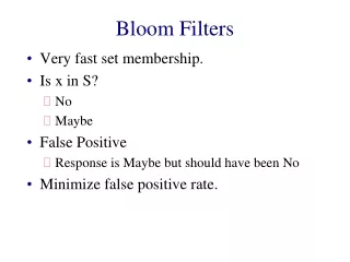
Key Y Filter DI Index N Y Y File DF Ans. Ideal Filter • Y=> this key is in the DI. • N=> this key is not in the DI. • Functionality of ideal filter is same as that of DI. • So, a filter that eliminates performance hit of DI doesn’t exist.
Key M BF DI N Index N Y Y File DF Ans. Bloom Filter (BF) • N=> this key is not in the DI. • M (maybe)=> this key may be in the DI. • Filter error. • BF says Maybe. • DI says No.
Key M BF DI N Index N Y Y File DF Ans. Bloom Filter (BF) • Filter error. • BF says Maybe. • DI says No. • BF resides in memory. • Performance hit paid only when there is a filter error.
Longest Matching Prefix • Suppose the router prefixes have W different lengths. • Create W Bloom filters, one for each length. • ith Bloom filter is for prefixes of length i. • Keep W hash tables. ith hash table has length i prefixes together with next hop information. • Query Bloom filters to get list of hash tables that may have matching prefix. • Query hash tables in decreasing order of length (or, in parallel) to find longest matching prefix.
… On Chip B1 B2 B3 BW … Off Chip H1 H2 H3 HW Longest Matching Prefix
Bloom Filter Design • Use m bits of memory for the BF. • Larger m => fewer filter errors. • When DI empty, all m bits = 0. • Use h > 0 hash functions: f1(), f2(), …, fh(). • When key k inserted into DI, set bits f1(k), f2(k), …, and fh(k) to 1. • f1(k), f2(k), …, fh(k) is the signature of key k.
1 1 1 1 0 0 0 0 0 0 0 0 0 0 1 2 3 4 5 6 7 8 9 0 0 Example • m = 11 (normally, m would be much much larger). • h = 2 (2 hash functions). • f1(k)= k mod m. • f2(k)= (2k) mod m. • k = 15. • k = 17.
1 1 1 1 0 0 0 0 0 0 0 0 0 0 1 2 3 4 5 6 7 8 9 0 0 Example • DI has k = 15 and k = 17. • Search for k. • f1(k)= 0 or f2(k)= 0 => k not in DI. • f1(k)= 1 and f2(k)= 1 => k may be in DI. • k = 6=> filter error.
Bloom Filter Design • Choose m (filter size in bits). • Use as much memory as is available. • Pick h (number of hash functions). • h too small => probability of different keys having same signature is high. • h too large => filter becomes filled with ones too soon. • Select the h hash functions. • Hash functions should be relatively independent.
Optimal Choice Of h • Probability of a filter error depends on: • Filter size … m. • # of hash functions … h. • # of updates before filter is reset to 0 … u. • Insert • Delete • Change • Assume that m and u are constant. • # of master file records = n >> u.
Probability Of Filter Error • p(u) = probability of a filter error after u updates = A * B • A = p(request for an unmodified record after u updates) • B = p(filter bits are all 1 for this request for an unmodified record)
A = p(request for unmodified record) • p(update j is for record i) = 1/n. • p(record i not modified by update j) = 1 – 1/n. • p(record i not modified by any of the u updates) = (1 – 1/n)u = A.
B = p(filter bits are all 1 for this request) • Consider an update with key K. • p(fj(K) != i) = 1 – 1/m. • p(fj(K) != i for all j) = (1 – 1/m)h. • p(bit i = 0 after one update) = (1 – 1/m)h. • p(bit i = 0 after u updates) = (1 – 1/m)uh. • p(bit i = 1 after u updates) = 1 – (1 – 1/m)uh. • p(signature of K is 1 after u updates) = [1 – (1 – 1/m)uh]h = B.
Probability Of Filter Error • p(u) = A * B = (1 – 1/n)u *[1 – (1 – 1/m)uh]h • (1 – 1/x)q ~ e–q/x when x is large. • p(u) ~ e–u/n(1 – e–uh/m )h • d p(u)/dh = 0 => h = (ln 2)m/u ~ 0.693m/u.
p(u) ~ e–u/n(1 – e–uh/m )h p(u) hopt h Optimal h • h ~ 0.693m/u. • m = 106, u = 106/2 • h ~ 1.386 • Use h = 1 or h = 2. • m = 2*106, u = 106/2 • h ~ 2.772 • Use h = 2 or h = 3.