Decision Tree Learning
Decision Tree Learning. Learning Decision Trees (Mitchell 1997, Russell & Norvig 2003)

Decision Tree Learning
E N D
Presentation Transcript
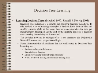
Decision Tree Learning • Learning Decision Trees (Mitchell 1997, Russell & Norvig 2003) • Decision tree induction is a simple but powerful learning paradigm. In this method a set of training examples is broken down into smaller and smaller subsets while at the same time an associated decision tree get incrementally developed. At the end of the learning process, a decision tree covering the training set is returned. • The decision tree can be thought of as a set sentences (in Disjunctive Normal Form) written propositional logic. • Some characteristics of problems that are well suited to Decision Tree Learning are: • Attribute-value paired elements • Discrete target function • Disjunctive descriptions (of target function) • Works well with missing or erroneous training data
Decision Tree Learning (Outlook = Sunny Humidity = Normal) (Outlook = Overcast) (Outlook = Rain Wind = Weak) [See: Tom M. Mitchell, Machine Learning, McGraw-Hill, 1997]
Day Outlook Temperature Humidity Wind PlayTennis D1 Sunny Hot High Weak No D2 Sunny Hot High Strong No D3 Overcast Hot High Weak Yes D4 Rain Mild High Weak Yes D5 Rain Cool Normal Weak Yes D6 Rain Cool Normal Strong No D7 Overcast Cool Normal Strong Yes D8 Sunny Mild High Weak No D9 Sunny Cool Normal Weak Yes D10 Rain Mild Normal Weak Yes D11 Sunny Mild Normal Strong Yes D12 Overcast Mild High Strong Yes D13 Overcast Hot Normal Weak Yes D14 Rain Mild High Strong No Decision Tree Learning [See: Tom M. Mitchell, Machine Learning, McGraw-Hill, 1997]
Decision Tree Learning • Building a Decision Tree • First test all attributes and select the one that would function as the best root; • Break-up the training set into subsets based on the branches of the root node; • Test the remaining attributes to see which ones fit best underneath the branches of the root node; • Continue this process for all other branches until • all examples of a subset are of one type • there are no examples left (return majority classification of the parent) • there are no more attributes left (default value should be majority classification)
Decision Tree Learning • Determining which attribute is best (Entropy & Gain) • Entropy (E) is the minimum number of bits needed in order to classify an arbitrary example as yes or no • E(S) = ci=1 –pi log2 pi , • Where S is a set of training examples, • c is the number of classes, and • pi is the proportion of the training set that is of class i • For our entropy equation 0 log2 0 = 0 • The information gain G(S,A) where A is an attribute • G(S,A) E(S) - v in Values(A) (|Sv| / |S|) * E(Sv)
Decision Tree Learning • Let’s Try an Example! • Let • E([X+,Y-]) represent that there are X positive training elements and Y negative elements. • Therefore the Entropy for the training data, E(S), can be represented as E([9+,5-]) because of the 14 training examples 9 of them are yes and 5 of them are no.
Decision Tree Learning:A Simple Example • Let’s start off by calculating the Entropy of the Training Set. • E(S) = E([9+,5-]) = (-9/14 log2 9/14) + (-5/14 log2 5/14) • = 0.94
Decision Tree Learning:A Simple Example • Next we will need to calculate the information gain G(S,A) for each attribute A where A is taken from the set {Outlook, Temperature, Humidity, Wind}.
Decision Tree Learning:A Simple Example • The information gain for Outlook is: • G(S,Outlook) = E(S) – [5/14 * E(Outlook=sunny) + 4/14 * E(Outlook = overcast) + 5/14 * E(Outlook=rain)] • G(S,Outlook) = E([9+,5-]) – [5/14*E(2+,3-) + 4/14*E([4+,0-]) + 5/14*E([3+,2-])] • G(S,Outlook) = 0.94 – [5/14*0.971 + 4/14*0.0 + 5/14*0.971] • G(S,Outlook) = 0.246
Decision Tree Learning:A Simple Example • G(S,Temperature) = 0.94 – [4/14*E(Temperature=hot) + 6/14*E(Temperature=mild) + 4/14*E(Temperature=cool)] • G(S,Temperature) = 0.94 – [4/14*E([2+,2-]) + 6/14*E([4+,2-]) + 4/14*E([3+,1-])] • G(S,Temperature) = 0.94 – [4/14 + 6/14*0.918 + 4/14*0.811] • G(S,Temperature) = 0.029
Decision Tree Learning:A Simple Example • G(S,Humidity) = 0.94 – [7/14*E(Humidity=high) + 7/14*E(Humidity=normal)] • G(S,Humidity = 0.94 – [7/14*E([3+,4-]) + 7/14*E([6+,1-])] • G(S,Humidity = 0.94 – [7/14*0.985 + 7/14*0.592] • G(S,Humidity) = 0.1515
Decision Tree Learning:A Simple Example • G(S,Wind) = 0.94 – [8/14*0.811 + 6/14*1.00] • G(S,Wind) = 0.048
Decision Tree Learning:A Simple Example • Outlook is our winner!
Decision Tree Learning:A Simple Example • Now that we have discovered the root of our decision tree we must now recursively find the nodes that should go below Sunny, Overcast, and Rain.
Decision Tree Learning:A Simple Example • G(Outlook=Rain, Humidity) = 0.971 – [2/5*E(Outlook=Rain ^ Humidity=high) + 3/5*E(Outlook=Rain ^Humidity=normal] • G(Outlook=Rain, Humidity) = 0.02 • G(Outlook=Rain,Wind) = 0.971- [3/5*0 + 2/5*0] • G(Outlook=Rain,Wind) = 0.971
Decision Tree Learning:A Simple Example • Now our decision tree looks like:
Decision Trees:Other Issues • There are a number of issues related to decision tree learning (Mitchell 1997): • Overfitting • Avoidance • Overfit Recovery (Post-Pruning) • Working with Continuous Valued Attributes • Other Methods for Attribute Selection • Working with Missing Values • Most common value • Most common value at Node K • Value based on probability • Dealing with Attributes with Different Costs
Decision Tree Learning:Other Related Issues • Overfitting when our learning algorithm continues develop hypotheses that reduce training set error at the cost of an increased test set error. • According to Mitchell, a hypothesis, h, is said to overfit the training set, D, when there exists a hypothesis, h’, that outperforms h on the total distribution of instances that D is a subset of. • We can attempt to avoid overfitting by using a validation set. If we see that a subsequent tree reduces training set error but at the cost of an increased validation set error then we know we can stop growing the tree.
Decision Tree Learning:Reduced Error Pruning • In Reduced Error Pruning, • Step 1. Grow the Decision Tree with respect to the Training Set, • Step 2. Randomly Select and Remove a Node. • Step 3. Replace the node with its majority classification. • Step 4. If the performance of the modified tree is just as good or better on the validation set as the current tree then set the current tree equal to the modified tree. • While (not done) goto Step 2.
Decision Tree Learning:Other Related Issues • However the method of choice for preventing overfitting is to use post-pruning. • In post-pruning, we initially grow the tree based on the training set without concern for overfitting. • Once the tree has been developed we can prune part of it and see how the resulting tree performs on the validation set (composed of about 1/3 of the available training instances) • The two types of Post-Pruning Methods are: • Reduced Error Pruning, and • Rule Post-Pruning.
Decision Tree Learning:Rule Post-Pruning • In Rule Post-Pruning: • Step 1. Grow the Decision Tree with respect to the Training Set, • Step 2. Convert the tree into a set of rules. • Step 3. Remove antecedents that result in a reduction of the validation set error rate. • Step 4. Sort the resulting list of rules based on their accuracy and use this sorted list as a sequence for classifying unseen instances.
Decision Tree Learning:Rule Post-Pruning • Given the decision tree: • Rule1: If (Outlook = sunny ^ Humidity = high ) Then No • Rule2: If (Outlook = sunny ^ Humidity = normal Then Yes • Rule3: If (Outlook = overcast) Then Yes • Rule4: If (Outlook = rain ^ Wind = strong) Then No • Rule5: If (Outlook = rain ^ Wind = weak) Then Yes
Decision Tree Learning:Other Methods for Attribute Selection • The information gain equation, G(S,A), presented earlier is biased toward attributes that have a large number of values over attributes that have a smaller number of values. • The ‘Super Attributes’ will easily be selected as the root, result in a broad tree that classifies perfectly but performs poorly on unseen instances. • We can penalize attributes with large numbers of values by using an alternative method for attribute selection, referred to as GainRatio.
Decision Tree Learning:Using GainRatio for Attribute Selection • Let SplitInformation(S,A) = - vi=1 (|Si|/|S|) log2 (|Si|/|S|), where v is the number of values of Attribute A. • GainRatio(S,A) = G(S,A)/SplitInformation(S,A)
Decision Tree Learning:Dealing with Attributes of Different Cost • Sometimes the best attribute for splitting the training elements is very costly. In order to make the overall decision process more cost effective we may wish to penalize the information gain of an attribute by its cost. • G’(S,A) = G(S,A)/Cost(A), • G’(S,A) = G(S,A)2/Cost(A) [see Mitchell 1997], • G’(S,A) = (2G(S,A) – 1)/(Cost(A)+1)w [see Mitchell 1997]