Download

1 / 20
200 likes | 302 Views
E. R. V. S. I. I. N. T. U. Y. O. H. F. T. U. P. O. L. M. Y. MANAGING WATER QUALITY OF S.W. EUROPEAN MARINE SITES (SEPT 03). Monitoring and modelling nutrients in catchments. Prof Paul Worsfold Biogeochemistry & Environmental Analytical Chemistry Group

E N D
E R V S I I N T U Y O H F T U P O L M Y MANAGING WATER QUALITY OF S.W. EUROPEAN MARINE SITES (SEPT 03) • Monitoring and modelling nutrients in catchments Prof Paul Worsfold Biogeochemistry & Environmental Analytical Chemistry Group Plymouth Environmental Research Centre University of Plymouth, UK email pworsfold@plymouth.ac.uk PERC PERC
Environmental monitoring • Objective: Provide high quality analytical data to: • Elucidate environmental processes and biogeochemical cycles • Monitor compliance with legislation, e.g. WFD • Archive data and provide baseline surveys e.g. EIA • Study chemical fluxes, pathways and fates • BUT sampling is expensive and time consuming • AND sample integrity may be lost • THEREFORE we need in situ monitoring
In situ environmental monitoring • Provides high quality data with excellent temporal and spatial resolution for process studies, catchment management and mapping but requires: • Rugged, portable, automated instrumentation • Contamination free environment • Reagents, containers, sampling apparatus, ship • Sensitive and selective detection • Removal of matrix interferences e.g. sea salts • Stability (reagents, standards, pumps, detector,) • Filtration and prevention of biofouling • Regular on-site calibration, maintenance & communication • THEREFORE WE NEED FLOW INJECTION ANALYSIS
600 Lough Conn, Ireland (1995-1997) 500 400 TP kgP/day 300 200 100 0 Apr-95 Apr-96 Apr-97 Aug-95 Aug-96 Aug-97 Oct-95 Oct-96 Oct-97 Jun-95 Jun-96 Jun-97 Dec-94 Dec-95 Dec-96 Dec-97 Feb-95 Feb-96 Feb-97 Temporal changes in river TP load • Periodic sampling ok for estimating annual loads. • However 90% of flow occurs in 10% of time. • Short term event driven pulses. • Diurnal cycles • Therefore need frequent analysis during these events to predict daily/monthly loads and study in-stream processes
Water Research 35 (2001) 3670 Storage effects for R. Frome P Fridge Chloroform Freezer Chloroform Fridge Control 2.0 4 4 3 3 1.5 PO4 -P (uM) PO4 -P (uM) PO4 -P (uM) 2 2 1.0 1 1 0.5 0 0 0.0 0 20 40 60 80 0 20 40 60 80 0 20 40 60 80 Day Day Day Fridge Freezer Deep Freezer 4 4 4 3 3 3 PO4 -P (uM) PO4 -P (uM) PO4 -P (uM) 2 2 2 1 1 1 0 0 0 0 20 40 60 80 0 20 40 60 80 0 20 40 60 80 Day Day Day
RESPONSE TIME (s) ACA 361 (1998) 63 Submersible Nitrate Manifold 260 ul sample injected via 5 um filter Packed reduction column -1 ml min Ammonium chloride Flow cell 0.32 (10 g l-1) 1 m reaction coil Mixed colour reagent 0.16 20 mm path: LOD 2.8 ug L-1 N Linear range 5 - 100 10 mm path: LOD 85 ug L-1 N Linear range 100 - 2500
Submersible Monitor Specifications • Tidal cycle (13 h), diurnal cycle (24 h) and transect deployment with high frequency • Submersible to 50 m (mixed layer) • Multiparameter e.g. nitrate & phosphate • Detection limit 0.1 M N (oligotrophic waters) • Rugged (protected cage), compact and light • Variable operational modes e.g. event triggered • Communication with base station • On-board filtration & calibration
Paulo Gardolinski Feb 2001 Submersible deployment Protective cage and reagents Pressure housing FI manifold
Talanta 58 (2002) 1015 North Sea surface nitrate mapping ug L-1 Nitrate 31 Dogger Bank 72.0 25 64.0 27 23 29 54.50 56.0 20 24 21 26 48.0 22 32 19 54.00 28 North Sea 18 40.0 11 10 12 17 33 32.0 9 13 7 34 8 53.50 Humber Estuary 24.0 14 6 15 3 16.0 4 2 5 53.00 The Wash 8.0 England 0.0 1 0.50 1.00 1.50 2.00 2.50
Integrated Chemical/Biological Monitor CAPMON Computer Computer Physical probes logger Sample Landfill leachate from Chelson Meadow waste treatment facility Ammonia Computer Test organisms - crayfish (Pacifastacus leniusculus) Holding tank Overflow Pump
Ecotoxicology 8 (1999) 225 Relation between ammonia and heart rate Maximum Heart rate (bpm) of P. Leniusculus (n=12) 160 120 80 40 0.1 Control 1.0 5.0 15 30 Ammonia (mg l-1)
Talanta 58 (2002) 1043 High temporal resolution P monitoring
25 200 30 a b c 175 25 20 1976 2000 1976 1996 150 1989 2000 1998 1987 1974 1999 1979 20 1989 1984 1998 1979 1992 15 125 1976 1993 1996 1986 1990 1997 1999 1999 1979 2000 1974 1974 1992 2002 1990 1992 1981 15 1990 1980 1987 100 1981 1988 1987 1985 1993 1980 1985 1981 1988 1998 2000 TEM (C) 10 1981 RAI (mm/day) FLW (m3/S) 2000 1974 1997 1990 1988 1990 1993 1978 1993 1983 1997 1982 1986 1976 75 1998 10 1981 1994 1998 2000 1993 1981 1987 1979 1992 2000 1988 1985 1986 1983 1984 1988 1986 1993 1985 1999 1978 1985 1979 1987 1993 1975 1986 1985 5 1983 50 2000 1998 1980 5 1986 1986 1985 1994 2000 1981 1999 1986 1988 1986 1993 1981 1996 1983 1981 1986 1992 1993 1983 1993 1993 25 1985 1994 1974 1977 1979 1985 1981 1993 1988 1993 1991 1992 1980 1993 1985 1985 1991 1979 1993 1998 1998 1986 1981 1998 1985 1979 1974 1986 0 1986 1992 1991 1988 0 1980 1981 1997 1993 1998 1987 1988 0 -5 -5 -25 W01 W06 W11 W16 W21 W26 W31 W36 W41 W46 W51 W01 W06 W11 W16 W21 W26 W31 W36 W41 W46 W51 W01 W06 W11 W16 W21 W26 W31 W36 W41 W46 W51 week week week 1990 1981 1989 1998 1.0 .2 1988 7 e f 1983 6 d 1976 1995 1989 .8 1976 1978 1997 1996 1976 1979 1996 5 1978 1997 1978 1996 .6 1976 1981 1974 4 1984 1991 1996 1983 1996 1976 1979 1983 PHO (mg/L) .4 NIT (mg/L) 1985 3 1985 1997 1998 1990 1996 1986 1990 1981 1991 1988 2 1994 1983 .2 1990 1981 1989 1998 1988 1986 1976 1995 1989 1978 1979 1978 1978 1995 1981 1984 1991 1979 1990 1996 1986 1 1981 1986 1983 1986 1986 1986 1980 1987 1976 1992 1996 0.0 1984 1988 1976 1980 1987 1991 1989 0 1992 1996 1984 1988 0.0 -.2 -1 N = 11 9 17 10 11 15 15 14 11 13 17 17 16 10 14 14 12 6 9 17 15 15 9 16 15 13 13 18 15 8 10 11 18 10 15 10 12 13 9 6 14 16 17 15 12 14 19 10 17 15 12 3 1 W01 W06 W11 W16 W21 W26 W31 W36 W41 W46 W51 W01 W06 W11 W16 W21 W26 W31 W36 W41 W46 W51 W01 W07 W13 W19 W25 W31 W37 W43 W49 W04 W10 W16 W22 W28 W34 W40 W46 W52 week week 1993 1974 150 600 175 1974 1977 g i 1990 1988 1995 h 1984 1988 1977 1974 1991 125 150 1974 1994 500 1988 1976 1980 1977 1993 1985 1992 100 1978 125 1998 1984 1989 1985 1994 1996 1979 400 1987 1981 1976 1986 1986 1977 75 100 1992 1977 1985 1983 1990 1979 1977 SS (mg/L) 300 CHL (microg/L) 1981 1992 1978 1979 1990 1977 1987 50 1986 1985 1988 75 1997 1984 1984 1975 1986 1985 1988 1978 1981 1977 1974 1979 1986 1975 1985 1980 1992 1993 1976 200 1977 1986 1977 1976 1989 1975 25 1974 1975 1975 1996 50 1984 1981 1981 1980 1994 1993 1985 1977 1985 1976 1993 1974 1993 1979 1997 1984 1986 1994 1974 1994 1986 1977 1978 1988 1995 1986 1977 1988 1980 1974 1991 1986 1988 1974 1994 1992 1980 1977 100 1993 1985 1992 1978 0 1974 1998 1984 1985 1989 1994 1979 25 1981 1987 1976 1981 1986 1986 1977 1977 1992 1985 1990 1979 1977 1984 1981 1992 1979 1997 1982 1987 1986 1985 1988 1975 1997 1986 1985 1988 1981 1977 1978 1975 1974 1979 1985 1980 1992 1980 1982 1986 1995 1995 1989 1977 1975 1981 1974 1980 -25 1976 1985 1993 1979 1985 1997 1993 1986 1994 0 1984 1974 0 1986 1978 1986 1980 1986 1974 N = 16 15 19 13 13 18 16 17 13 17 19 19 19 14 19 19 16 11 12 21 18 20 14 21 18 18 17 21 18 12 15 16 21 14 20 13 17 17 14 11 16 19 20 18 16 17 22 14 19 20 15 7 3 W01 W06 W11 W16 W21 W26 W31 W36 W41 W46 W51 W01 W06 W11 W16 W21 W26 W31 W36 W41 W46 W51 W01 W07 W13 W19 W25 W31 W37 W43 W49 W04 W10 W16 W22 W28 W34 W40 W46 W52 week week Historical Tamar data • Rainfall • Flow • Temperature • Phosphate • Nitrate • Suspended solids • Chlorophyll
Modelled Tamar data 1974 - 1998 Nitrate + nitrite Phosphate
Export Coefficients for ITE Land Cover Types Export coeff. -1 ITE grid Landcover type % catchment kg P y (kg ha-1 y-1) code area 1 Sea / Estuary 0.00 0.00 0 2 Inland water 0.02 0.00 0 3 Beach and Coastal bare 0.00 0.00 0 4 Saltmarsh 0.00 0.00 0 5 Grass heath 1.27 0.02 10.5 6 Mown / Grazed turf 19.4 0.20 1611 7 Meadow/Verge/Semi-natural 31.0 0.20 2563 8 Rough / Marsh grass 0.98 0.02 8.10 12 Bracken 0.0005 0.02 0.004 13 Dense shrub heath 0.50 0.02 4.22 14 Scrub / Orchard 0.92 0.02 7.64 15 Deciduous woodland 7.37 0.02 61.0 16 Coniferous woodland 2.64 0.02 21.9 18 Tilled land 28.0 0.66 7666 20 Suburban / Rural dev. 4.32 0.83 1486 21 Continuous urban 0.19 0.83 65.8 22 Inland bare ground 0.52 0.70 151 24 Lowland bog 0.10 0.00 0 25 Open shrub heath 0.63 0.02 5.22 Unclassified 2.13 0.48 424 Total 100 14,085
Nutrient source Export coefficients -1 kg P y Animals: Horses 2.85 % 27 Cattle 2.85 % 330 Pigs 2.55 % 713 Sheep 3.00 % 250 Total1,320 Humans: Sewage systems 0.38 kg P capita 8,869 -1 -1 y Septic systems 0.24 kg P capita 1,331 -1 -1 y Total 10,200 Export Coefficients for Animal Waste and Population Equivalents Total export modeled 25,605
J. Env. Qual. 30 (2001) 1738 GIS of Frome catchment land use Modelled export (1998) 25,605 kg y-1 P Observed export (1998) 23,400 kg y-1 P GIS plot prepared by Grady Hanrahan & Gordon Irons
Phosphorus reduction scenarios for STWs within the Frome catchment Implementation of phosphorus removal technology (Urban Wastewater Directive) All data in kg P y-1 Dorchester All STWs Total Original 4942 8869 25605 Treatment at 2768 6695 23431 Dorchester STW Treatment at 2768 4967 21703 all STWs
Ian McKelvie & Paulo Gardolinski Organic P release from sediment
Nutrient monitoring & modelling • Reliable field instrumentation for in situ monitoring and ground truthing models • High temporal resolution for studying in stream processes (diurnal, storm event) • High spatial monitoring for global mapping • Integration with ecotoxicological monitoring • PLS models of large historical data sets • Empirical models based on export coefficients • Respond to policy drivers e.g. Water Framework Directive