Understanding Gamma-Ray Bursts: Concepts, Phenomenology, and Observations
This overview explores Gamma-Ray Bursts (GRBs), brief but intensely energetic flashes of gamma radiation originating from cosmic events. We discuss the electromagnetic waves associated with GRBs, their redshift measurements indicating distance, and the key differences between short and long GRBs. The historical context of GRB discovery, particularly by American satellites in the 1960s, is examined, alongside their energetic phenomena, isotropic sky distribution, and the significance of afterglows. Insights into GRB origins, including collapsars and neutron star mergers, highlight their importance in astrophysical research.

Understanding Gamma-Ray Bursts: Concepts, Phenomenology, and Observations
E N D
Presentation Transcript
The waves perturbation Direction of propagation
ELETTROMAGNETIC WAVE Continuum series of pulses originated from a variation of the electromagnetic field. It is a perturbation of the electromagnetic field.
The redshift and the distance Measurement redshift: The light frequency is lower than the frequency was emitted. This happens when the source is receding in the observer We look at the spectrum of an electromagnetic light emission of an object and we compare it with another nearer SUN GALAXY
Gamma-Ray Bursts: The story begins The Vela are American satellites that try to see if the URSS respects the Treats banning nuclear tests between USA and URSS in the early 60s Brief, intense flashes of g-rays They were too much long to be nuclear explosions and too much short to be a known phenomenon! Klebesadel R.W., Strong I.B., Olson R., 1973, Astrophysical Journal, 182, L85 `Observations of Gamma-Ray Bursts of Cosmic Origin’
GRBs phenomenology Basic phenomenology • Flashes of high energy photons in the sky (typical duration is few seconds). • Isotropic distribution in the sky • Cosmological origin accepted (furthest GRBs observed z ~ 7 – billions of light-years). • Extremely energetic and short: the greatest amount of energy released in a short time (not considering the Big Bang). • Sometimes x-rays and optical radiation observed after days/months (afterglows), distinct from the main γ-ray events (the prompt emission). • Observed non thermal spectrum
The energetics of GRBs An individual GRB can release in a matter of seconds the same amount of energy that our Sun will radiate over its 10-billion-year lifetime
Short GRBs-> T90<5 s Long GRBs-> T90>5 s Short vs Long GRBs Short (hard) Long (soft) ShortGRBs -> T90<2 s Long GRBs -> T90>2 s Kouveliotou et al., 1996, AIP Conf. Proc., 384, 42. Paciesas et al., 1999, ApJS, 122, 465. Donaghy et al., 2006, astro-ph/0605570. Norris et Bonnell 2006
What is the T90 • Time interval in which the instrument reveal the 5% of the total counts and the 90%. • To the duration of this event it is associated the 90% of the emission
compact object mergers (NS-NS, NS-BH) short GRBs Progenitors for traditional model core collapse of massive stars (M > 30 Msun) long GRBs Collapsar or Hypernova(MacFadyen & Woosley 1999 Hjorth et al. 2003; Della Valle et al. 2003, Malesani et al. 2004, Pian et al. 2006) GRB simultaneous with SN Discriminants: host galaxies, location within host, duration, environment, redshift distribution, ...
Very massive star that collapses in a rapidly spinning BH. • Identification with SN explosion. Woosley (1993)
prompt emission FRED (Fast Rise, Exponential Decay)
Pre-Swift vs Swift for the afterglows Swift zmedio = 2.5!!! Pre-Swift zmedio = 1.2 Typical lightcurve for BeppoSAX Typical lightcurve for Swift
Definition of the Flux and Energy • The flux F is the energy carried by all rays passing through a given area dA . • dA normal to the direction of the given ray • all rays passing through dA whose direction is within a solid angle dΩ of the given ray • E=Iν *dA*dt*dΩ*dν • Iv= is the brightness or specific intensity • dFν =E/(dA*dt*dν) • dF= For some arbitrary orientation n
Gamma-ray Burst Real-time Sky Map http://grb.sonoma.edu/ • Burst List • Burst ID GRB 090301A • Date 2009/03/01 • Time 06:55:55 • Mission Swift • RA 22:32 • Dec 26:38 • brief Burst Description This burst had a complex multipeak structure and a duration of ~50 seconds. Due to observing constraints Swift cannot slew to this position until after April 15. No XRT or UVOT was available as a result.
Eα N(E) Eβ Ebreak E Spectra Non thermal spectra Epeak =(α +2) Ebreak α~-1 β~ -2 Ebreak ~ 100 keV - MeV The phenomenological Band law hold in a wide energy interval 2keV-100MeV
Epeak featureless continuum power-laws - peak in F F ~ Eb F ~ Ea GRB spectrum evolves with time within single bursts Hard to soft evolution cts/sec This coefficient α in the L-Ta analysis it is βa (so it will be call the same in the exercise) Time [sec]
, Surf. Jet half opening angle Relativistc beaming: emitting surface 1/ Log(F) Jet break Log(t) Jet effect >> 1/ 1/
X-ray Flashes and X-ray Rich Bursts • XRFs prompt emission spectrum peaks at energies tipically one order of magnitude lower than those of GRBs. XRFs empirically defined by a greater fluence in the X-ray band (2-30keV) than in the γ-ray band (30-400keV). • XRR are an intermediate class between XRFs and GRBs
Why GRBs are so studied for the correlations? GRBs are extremely energetic events and are expected to be visible out to z ~ 15-20 (Lamb & Reichart, 2000, ApJ, 536, 1), which is further than that obtainable by quasars (zmax ~ 6). GRB z ~ 6.7 (Tagliaferri et al. 2005) Potential use of GRBs to derive an extended z Hubble-diagram.
Peak energy – Isotropic energy Correlation 9+2 BeppoSAX GRBs Epeak Eiso0.5 Amati et al. 2002 Epeak(1+z)
+ 21 GRBs (Batse, Hete-II, Integral) Ghirlanda, Ghisellini, Lazzati 2004 Amati 2006 (most recent update) Epeak Eiso0.5 X2=357/28 Epeak(1+z) Eiso
1- cos qjet “Ghirlanda” (25) “Amati” (62) Nava et al. 2006; Ghirlanda et al. 2007 Why is the Ghirlanda relation, Eg (Epeak) 1.5, different from the Amati relation, Eiso Epeak 0.5 ? Because of the correction of the beaming angle
A completely empirical correlation between prompt (Ep, Eiso) and afterglow properties (tbreak) (Liang & Zhang 2005) Model dependent: uniform jet + wind density Model dependent: uniform jet + homogeneous density Through simple algebra it can be verified that the model dependent correlations are consistent with the empirical correlation! (Nava et al. 2006)
… still not convinced ? … A new correlation between Liso, Ep, T0.45 Good fit Consistent with other corr ONLY PROMPT EMISSION PROPERTIES Firmani et al. 2006
The study of prompt vs afterglow A further step to build LX –Ta relation A lot of kinetic energy should remain to power the afterglow Prompt SAX X-ray afterglow light curve Piro astro-ph/0001436
Eafterglow < Eprompt Eafterglow ~ 0.1 Eprompt
Flux vs observed time s=0.48 Nardini et al. 2006
Clustering of the optical luminosities Luminosity vs rest frame time s=0.28 Nardini et al. 2006
GRB – Afterglow – Temporal Properties GRB multiwavelength emission Panaitescu & Kumar
LX-Eg correlate in optical and in X? No corr.
The X-ray luminosities are more widely used for testing correlations We also choosed X-ray luminosity for our analysis
Why we are searching a new correlation? • to find a relation involving an observable property to standardize GRBs • in the same way as the Phillips law with SNeIa
The sample • 17 GRBs with 0.0085< z<1.949 (Swift, BeppoSAX, Integral) Ltotal= Cg(t) = kh(t) + atb = L1 + L2 (1) g(t) is the temporal shape of the whole lightcurve h(t) t< tstart g(t)= atbstartt > tstart For g(tstart) = atbstart =kh(tstart) Integrating 1) Normalization • C=Etot
Focusing on L2 • L2= Linearization provides a visual evidence of the claimed model and it gives the quantities as logarithms ready to compute the distance moduli Linear fits are used to find parameters also of other models which can be linearized through a suitable transformation of the variables. Non-linear least-squares (NLLS) Marquardt-Levenberg algorithm, .a and b computed by the fit. Values for -1.17 < b < -1.91
The tbreakof the lightcurve is highly variable 103<tstart<104s The Spearman coefficient of correlation is 0.75 The correlation is new because it involves only the afterglow quantities How can we improve it? Increasing the statistic of GRBs observed by the same instruments to see if there is a selection effect depending on the instruments and improving the statistical method We used Ta and Fa values computed through Willingale et al. 2007 of the afterglow and the D’Agostini method as statistical method.
SWIFT Willingale et al. 2007
(Tc, Fc) is the transition between the exponential and the power law αc the time constant of the exponential decay, Tc/αc • tc marks the initial time rise and the time of maximum flux occurring at In most cases ta=Tp. No case in which thetwo componetswere sufficiently separated such that this time could be fitted as a free parameter. We are unable to see the rise of the afterglow component because the prompt component always dominates at early times and ta could be much less than Tp for most GRBs.
1)f_c(t) = f_p(t) + f_a(t) 2)f_p(t)= fa(t)= The phenomenological formula For t<Ta Negligible if ta=0 and in that case we return to the simple case of power law decay Willingale at al. 2007
General treatment 3) Lbol = 4 πDL2 (z) P bol Pbolo is the bolometric flux, while P is the peak flux, Emin-Emax is the energy range in which P occurs
We compute the X-ray luminosities at the time Ta so that we have to set f(t)=f (Ta)=fa(Ta) Since the contribution on the prompt component is typically smaller than the 5%, Much lower than the statistical uncertainty on Fa(Ta). Neglecting Fp(Ta) we reduce the error on Fx(Ta) without introducing any bias. 3) LX(Ta) = 4 πDL 2(z) FX(Ta)=aTab E_min, E_max = (0.3, 10) keV set by the instrument bandpass
Due to the limited energy range, the GRB spectrum may be described by a simple • power law • β(t) • βpfor the prompt phase • βpd for the prompt decay • βafor the plateau observed at the time Ta • βad for the afterglow at t > Ta We estimate βa because we compute Fx(Ta)
The sample Computing LX(Ta) requires βa and z Most of the 107 GRBs reported in Willingale 07 are discarded (no βa and z) 47 have z but not the whole sample have βa Reduced sample: 32 GRBs with both log LX(Ta) and log [Ta/(1+z)]
The computations errors • the parameters of interest are given with their 90%confidence ranges. • Following Willingale (priv. comm.), we have assumed independent Gaussian • errors and obtained 1 sigma uncertainties by roughly dividing by 1.65 the 90% errors.