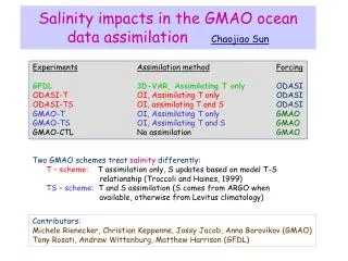
Data assimilation in the ocean

1. Data assimilation in the ocean Kristian S. Mogensen with input from the marine aspects and reanalysis sections

2. Outline of lecture • Ocean circulation and modelling in 2 slides. • Applications of ocean data assimilation: • Importance of ocean data assimilation on the coupled forecasts. • Ocean data assimilation and historical ocean reanalyses. • The ocean observing system • Deep ocean data assimilation systems • Background co-variances • Balance relationships for salinity and velocity • Altimeter assimilation • Bias correction • ECMWF’s current ocean assimilation system • Ocean reanalysis • A brief introduction to wave data assimilation • Future directions • Coupled data assimilation.

3. Ocean circulation: some facts • The radius of deformation in the ocean is small (~30km). So one expects things to happen on much smaller scales than in the atmosphere where the radius of deformation is ~3000km. • [Radius of deformation =c/f where c= speed of gravity waves. In the ocean c~<3m/s for baroclinic processes.] • The time scales for the ocean cover a much larger range than for the atmosphere: slower time scales for adjustment. • The ocean is strongly stratified in the vertical. • The ocean is forced at the surface by the wind, by heating/cooling and by fresh water fluxes (precip-evap). • For modelling this means that uncertainty in forcing fluxes contributes to uncertainty in model results. • The electromagnetic radiation does not penetrate into the ocean, which makes the deep ocean difficult to observe from satellites. • The surface of the ocean can however be observed from space.

4. Ocean modelling components: • The blue ocean: ocean dynamics. • Primary variables: potential temperature (T), salinity (S) current (U,V) and sea surface height (SSH). • Density is a function of T and S though the equation of state. • Typical a regression is used. • The white ocean: sea-ice. • The green ocean: biogeochemistry. • Ocean waves. • Coast lines and bathymetry can be major headaches. • Since ECMWF is not doing biochemistry modelling this will not be touched upon.

5. 3D ocean data assimilation

6. Why do we do deep ocean analyses? • Climate Resolution (global ~1x1 to 1/4x1/4 degrees) • To provide initial conditions for seasonal forecasts. • To provide initial conditions for monthly forecasts • To provide initial conditions for multi-annual forecasts (experimental only at this stage) • To reconstruct the history of the ocean (re-analysis) • High resolution ocean analysis (regional, ~1/3-1/9-1/12 degrees) • To monitor and to forecast the state of the ocean Defence, commercial applications (oil rigs …)

7. Basis for extended range forecasts: monthly, seasonal, decadal • The forecast horizon for weather forecasting is a few days. Sometimes it is longer e.g. in blocking situations 5-10 days. • Sometimes there might be predictability even longer as in the intra-seasonal oscillation or Madden Julian Oscillation. • But how can you predict seasons, years or decades ahead? • The feature that gives longer potential predictability is forcing given by slow changes on boundary conditions, especially to the Sea Surface Temperature (SST) • Atmospheric responds to SST anomalies, especially large scale tropical anomalies • El Nino/Southern Oscillation is the main mode for controlling the predictability of the interannual variability.

8. Nino 3 Nino 3.4 SST variability is linked to the atmospheric variability suggesting a strongly coupled process. Sea Level Pressure (SOI) • In the equatorial Pacific, there is considerable interannual variability. • The EQSOI (INDO-EPAC) is especially useful: it is a measure of pressure shifts in the tropical atmosphere but is more representative than the usual SOI (Darwin – Tahiti). • Note 1983, 87, 88, 97, 98 . Sea Surface Temperature (Nino 3)

9. Atmospheric model Atmospheric model Wave model Wave model Ocean model from day 10 onwards (from day 0 later this year). Ocean model Ocean Analysis Ocean Analysis ECMWF: Weather and Climate Dynamical Forecasts 15-Day ENS Medium-Range Forecasts Seasonal Forecasts Monthly (32 days) Extension of ENS Twice Weekly

10. Elephant seals ARGO floats XBT (eXpandableBathiThermograph) Moorings Satellite SST Sea Level The Ocean Observing system

11. 1982 1993 2001 XBT’s 60’s Satellite SST Moorings/Altimeter ARGO TRITON 1998-1999 PIRATA Time evolution of the Ocean Observing System 2008 Gravity info: GRACE GOCE SSS info: Aquarius SMOS

12. Changes to the T/S obs. network • Very uneven distribution of observations. • Southern ocean poorly observed until ARGO period.

13. No. of T obs. as function of time

14. No. of S obs. as function of time

15. SSH observational coverage 20060101

16. No. of SSH obs. as function of time

17. Ocean assimilation systems • Can be based on optimum interpolation (OI), variational techniques (e.g. 3D/4D-Var) or various ensemble Kalman filter based methods. • Or various hybrid combinations. • Just like for the atmospheric systems. • How to deal with coast lines is not trivial. • E.g. we don’t want increments (result of analysis) from the Pacific to propagate to the Atlantic across Panama. • To avoid initialization shock increments are typically applied via Incremental Analysis Update (IAU) which applies the increments as a forcing term over a period of time.

18. Ocean assimilation systems 2 • In the following I will use the “NEMOVAR” assimilation system to illustrate the ocean assimilation process. • Variational system under development by CERFACS, ECMWF, INRIA and the Met Office for assimilation into the NEMO ocean model. • Solves a linearized version of the full non-linear cost function. • 3D-Var presently, but 4D-Var is under development. • This system has been adopted by ECMWF and the Met Office for operational ocean data assimilation. • Uses recursive filters for correlation model (not discussed here). • Most of the examples is for illustration only and not necessary the optimal way of assimilation. • Single observation experiments

19. Background errors for ocean assim. • Length scales for a typical climate model: • ~2 degree at mid latitudes • ~15-20 degrees along the eq. • The background error correlation scales are highly non isotropic to reflect the nature of equatorial waves- Equatorial Kelvin waves which travel rapidly along the equator ~2m/s but have only a limited meridional scale as they are trapped to the equator. • Complex structures an smaller length scales near coastlines are usually ignored. • Background errors are correlated between different variables (multivariate formulation) through balance relations (next slides). • E.g. an temperature observation gives rise to an increment in salinity. • The background errors can be flow dependent.

20. A linearized balance operator for global ocean assimilation Temperature Salinity Treated as approximately mutually independent without cross correlations SSH u-velocity v-velocity Density Pressure • Define the balance operator symbolically by the sequence of equations (Weaver et al., 2005, QJRMS)

21. Components of the balance operator Salinity balance (approx. T-S conservation) SSH balance (baroclinic) u-velocity balance (geostrophy with β-plane approx. near eq.) v-velocity (geostrophy, zero at eq.) Density (linearized eq. of state) Pressure (hydrostatic approx.)

22. Horizontal correlation of T at 100m • From single observation of temperature experiment. • Wide longitudinal length scales at equator. • At 50 N the coast line comes into play.

23. Horiz. cross correlation of T at 100m T S • From single observation of temperature experiment. • The specific background determines the shape due to the balance relations. • S, U, V, SSH increments are from balance with T only. U V SSH

24. Assimilation of T/S profiles • Profile in the Golf stream for NEMOVAR 1 deg setup

25. Sea Level anomaly Equatorial Temperature anomaly Sea Level Anomaly from Altimetry El Nino 1997/98

26. Assimilation of altimeter data Ingredients: • The Mean Sea Level is a separate variable, and can be derived from Gravity information from GRACE (Rio9 from CLS, NASA, …) and future GOCE. But the choice of the reference global mean is not trivial and the system can be quite sensitive to this choice. Active area of research. • The GLOBAL sea level changes can also assimilated: • Ocean models are volume preserving, and can not represent changes in GLOBAL sea level due to density changes (thermal expansion, ….). • The difference between Altimeter SL and Model Steric Height is added to the model as a fresh water flux. A Mean Sea Level Observed SLA (Sea Level Anomaly) from T/P+ERS+GFO Respect to 7 year mean of measurements

27. Horizontal cross correlation of SSH SSH T • From single observation of SSH experiment. • T, S, U, V increments are from the balance constraint at 100 m. • The SSH increments is the full increment (balanced+unbalanced). S U V

28. SLA issues • The SLA along track data has very high spatial resolution for the 1 degree “class” of ocean assimilation systems. • Features in the data which the model can not represent. • Illustrated on the next 2 slides. • This can be dealt with in at least two different ways: • Inflate the observation error to account for non representativeness of the “real” world in the assimilation system. • Construction of “superobs” by averaging.

29. SLA Observations in 10 days

30. SLA from the 1 deg NEMO model

31. Why a bias correction scheme? Bias Correction Scheme • A substantial part of the analysis error is correlated in time. • Changes in the observing system can be damaging for the representation of the inter-annual variability. • Part of the error may be induced by the assimilation process. What kind of bias correction scheme? • Multivariate, so it allows to make adiabatic corrections (Bell et al 2004) • It allows time dependent error (as opposed to constant bias). • First guess of the bias non zero would be useful in early days (additive correction rather than the relaxation to climatology in S2) • Generalized Dee and Da Silva bias correction scheme • Balmaseda et al 2007

32. PIRATA Impact of data assimilation on the mean Assim of mooring data CTL=No data Large impact of data in the mean state: Shallower thermocline

33. Effect of bias correction on the time-evolution Assim of mooring data CTL=No data Bias corrected Assim

34. ECMWF Operational Ocean Assimilation system: ORA-S4 • Main Objective: Initialization of coupled forecasts • Historical reanalysis brought up-to-date • Source of climate variability. • Main Features • ERA-40 daily fluxes (1959-1988), ERA-INTERIM fluxes (1989-) and NWP in NRT • Retrospective Ocean Reanalysis back to 1957 • Multivariate on-line Bias Correction • Assimilation of temperature, salinity, altimeter sea level anomalies and global sea level trends. • 3D VAR based on NEMOVAR • Balance constrains as previous discussed. • Sequential, 10 days analysis cycle, IAU

35. DataAssimilation improves the interannual variability of the ocean analysis Correlation with OSCAR currents Monthly means, period: 1993-2009 Seasonal cycle removed

36. Impact on ECMWF-S4 SST Seasonal Forecast Skill

37. Climate Signals: Ocean Heat Content Anomalies with respect to 1980 to 2005. Units:10**22J

38. Wave data assimilation

39. Assimilation of Wave Data • Assimilation Method for Altimeter data: • Data are subjected to a quality control process. • Simple optimum interpolation (OI) scheme on SWH. • The wave spectrum is adjusted based on the analysis increment. • Assimilation Method for SAR data: • SAR spectra are inverted to ocean wave spectra. • Ocean spectra are partitioned into wave systems which then paired with the corresponding systems in the model. • Simple OI scheme on integrated parameters of the systems. • Each partition is adjusted based on its analysis increment.

40. Assimilation of Wave Data • NRT Altimeter (Ku) SWH operational assimilation at ECMWF: - ERS-1 URA, 15 August 1993 – 1 May 1996; - ERS-2 URA, 1 May 1996 – 23 June 2003; - ENVISAT RA-2 FDMAR, 22 October 2003 – 7 April 2012; - Jason-1 OSDR, 1 February 2006 – 1 April 2010 (with a gap); - Jason-2 OGDR, 10 March 2009 – on-going • NRT SAR spectra operational assimilation at ECMWF:- ERS-2 SAR UWA, 13 January 2003 – 31 January 2006; - ENVISAT ASAR WVS, 1 February 2006 – 21 October 2010. 21 Oct. 2010 1 Feb. 2006 13 Jan. 2003 SAR ENVISAT ASAR ERS-2 SAR ERS-1 ERS-2 Jason-2 Envisat Jason-1Envisat Jason-2Envisat Jason-1 Jason-2Envisat Jason-2Envisat Alt. 15 Aug. 1993 1 May 1996 22 Oct. 2003 7Apr. 2012 10 Mar. 2009 8 Jun. 2009 1 Apr. 2010

41. Impact of Alt. SWH assimilation. Mean increments

42. Impact of Alt. SWH assimilation – Model Forecast Verified againstin-situ data Verified againstJason-2 data ENVISAT RA-2 Assimilation 1 Jan. - 31 March 2012

43. Future directions: Coupled data assimilation.

44. Motivations for coupled data assimilation • Basically: • Ocean models need improved surface fluxes • Atmospheric models need improved sea surface temperature • Coupled data assimilation should: • improve the use of near-surface observation data • improve the ocean/atmosphere balance • improve the prediction of extreme air-sea flux events • reduce coupling shocks in coupled forecasts

45. Coupled assimilation schemes • Fully coupled assimilation • coupled model for the nonlinear trajectories • balanced fields • one analysis calculated by one minimization process • balanced analysis • coupled adjoint for a 4D-VAR approach • modelisationof covariances between atmosphere and ocean • Weakly coupled assimilation • coupled model for the nonlinear trajectories • balanced fields • two analysis computed in parallel by two minimization processes • avoid the development of new adjoint codes • covariancesbetween atmosphere and ocean are not required • possible information exchange during the minimizations • potentially unbalanced analysis

46. Work in progress: CERA. • Weakly coupled data assimilation system initially intended for the reanalysis. • The atmosphere (IFS) runs coupled to the ocean (NEMO) in the “outer” loops (trajX). • The minimization of the cost function is done separately for the ocean and the atmosphere.

47. Summary • Data assimilation in the ocean serves a variety of purposes, from climate monitoring to initialization of coupled model forecasts. • Compared to the atmosphere, ocean observations are scarce. The main source of information are temperature and salinity profiles (ARGO/moorings/XBTs), sea level from altimeter, SST from satellite/ships and geoid from gravity missions. • Assimilation of ocean observations reduces the large uncertainty(error) due to the forcing fluxes. It also improves the initialization of seasonal forecasts, and it can provide useful reconstructions of the ocean climate. • Data assimilation changes the ocean mean state. Therefore, consistent ocean reanalysis requires an explicit treatment of the bias. More generally, we need a methodology that allows the assimilation of different time scales. • Data assimilation for the wave model is important for short lead times (days), whereas data assimilation for the 3D ocean is important for long lead times (months). • The separate initialization of the ocean and atmosphere systems can lead to initialization shock during the forecasts. A more balance “coupled” initialization is desirable, but it remains challenging.

48. Some references related to ocean data assimilation at ECMWF • Evaluation of the ECMWF ocean reanalysis system ORAS4, Balmaseda, M. A., Mogensen, K. and Weaver, A. T. (2012),. Q.J.R. Meteorol. Soc.. doi: 10.1002/qj.2063 • The NEMOVAR ocean data assimilation system as implemented in the ECMWF ocean analysis for System 4, Mogensen et al 2012. ECMWF Tech-Memo 668. • The ECMWF System 3 ocean analysis system, Balmaseda et al 2008. MWR. See also ECMWF Tech-Memo 508. • Three and four dimensional variational assimilation with a general circulation model of the tropical Pacific. Weaver, Vialard, Anderson and Delecluse. ECMWF Tech Memo 365 March 2002. See also Monthly Weather Review 2003, 131, 1360-1378 and MWR 2003, 131, 1378-1395. • NEMOVAR: A variational data assimilation system for the NEMO ocean model. Mogensen et al. ECMWF newsletter No. 120 Summer 2009. • Balanced ocean data assimilation near the equator. Burgers et al. J Phys Ocean, 32, 2509-2519. • Salinity adjustments in the presence of temperature adjustments. Troccoli et al., MWR.. • Comparison of the ECMWF seasonal forecast Systems 1 and 2. Anderson et al ECMWF Tech Memo 404.

49. Some references related to ocean data assimilation at ECMWF 2 • Sensitivity of dynamical seasonal forecasts to ocean initial conditions. Alves, Balmaseda, Anderson and Stockdale. Tech Memo 369. Quarterly Journal Roy Met Soc. 2004. February 2004 • A Multivariate Treatment of Bias for Sequential Data Assimilation: Application to the Tropical Oceans. Q. J. R. Meteorol. Soc., 2007. Balmaseda et al. • A multivariate balance operator for variational ocean data assimilation. Q.J.R.M.S, 2006, Weaver et al. • Salinity assimilation using S(T) relationships. K Haines et al Tech Memo 458. MWR, 2006. • Impact of Ocean Observing Systems on the ocean analysis and seasonal forecasts, MWR. 2007, Vidard et al. • Impact of ARGO data in global analyses of the ocean, GRL,2007. Balmaseda et al. • Historical reconstruction of the Atlantic Meridional Overturning Circulation from the ECMWF ocean reanalysis. GRL 2007. Balmaseda et al.