c onsulting engineers and scientists
720 likes | 1.14k Views
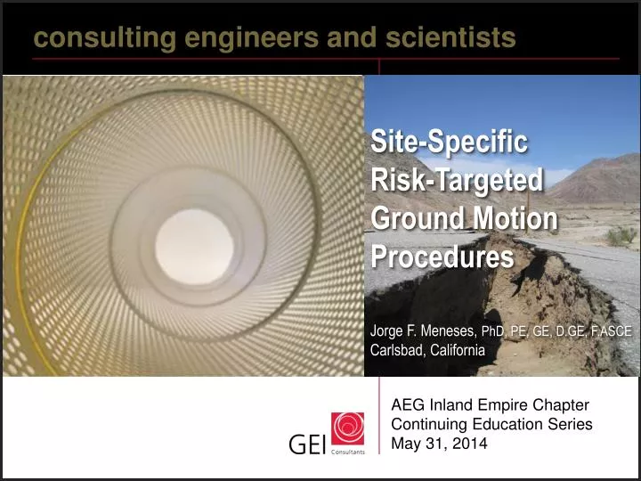
c onsulting engineers and scientists. Site-Specific Risk-Targeted Ground Motion Procedures Jorge F. Meneses, PhD, PE, GE, D.GE, F.ASCE Carlsbad, California. AEG Inland Empire Chapter Continuing Education Series May 31, 2014. Outline. Overview Site-specific procedures Risk coefficient

c onsulting engineers and scientists
E N D
Presentation Transcript
consulting engineers and scientists Site-Specific Risk-Targeted Ground Motion ProceduresJorge F. Meneses, PhD, PE, GE, D.GE, F.ASCECarlsbad, California AEG Inland Empire Chapter Continuing Education Series May 31, 2014
Outline • Overview • Site-specific procedures • Risk coefficient • NGA Relationships • Deaggregation • Examples • Performance Based EE • Summary
SITE-SPECIFIC STUDY • 2103 CBC, 1616.10.2, 1616A.1.3 “For buildings assigned to Seismic Design Category E and F, or when required by the building official, a ground motion hazard analysis shall be performed in accordance with ASCE 7 Chapter 21, as modified by Section 1803A.6 of this code.”
SITE-SPECIFIC STUDY (cont’d) Site Response Analysis • Structures on Site Class F sites (Ts > 0.5 seconds) • At least 5 recorded or simulated horizontal ground motion acceleration time histories (MCER spectrum at bedrock) Seismic Hazard Analysis • Seismically isolated structures (S1 0.6) • Structures with damping systems (S1 0.6) • A time history response analysis of the building is • performed (ASCE 7-10, Section 11.4.7, p.67)
SITE RESPONSE ANALYSIS Ground Surface Rock base (ASCE 7-10, Section 21.1, p.207)
SITE-SPECIFIC GROUND MOTION PROCEDURE • Probabilistic ground motion • Method 1: Uniform-hazard GM * Risk Coefficient • Method 2: Risk-targeted probabilistic GM directly • Deterministic ground motion • 84th-%ile GM, but not < 1.5Fa or 0.6*Fv/T • MCER = Min (Prob. GM, Det. GM) • All GMs are max-direction spectral accelerations (Sa) (Sections 21.2, 21.3, and 21.4)
Risk coefficient • Risk coefficient: CR • T ≤ 0.2 s; CR = CRS (Figure 22-17) • T ≥ 1.0 s; CR = CR1 (Figure 22-18) • 0.2 s ≤ T ≤ 1.0 s; CR linear interpolation of CRS and CR1
SITE-SPECIFIC GROUND MOTION PROCEDURE 1% Prob. of collapse 50 yr (direction of max horiz resp) 84th percentile (direction of max horizresp) Site Coord Site Class Prob MCER Det MCER Lesser of PSHA and DSHA General MCE Spectrum MCER Spectrum 2/3 MCE Spectrum 2/3 MCE Spectrum General DESIGN Spectrum DESIGN Spectrum > 80% General Design Spectrum SITE-SPECIFIC DESIGNSPECTRUM (Sections 21.2, 21.3, and 21.4)
SITE-SPECIFIC GROUND MOTION PROCEDURE Deterministic Lower Limit (DLL) on MCER Spectrum Sa (g) 1.5 Fa Sa = 0.6 Fv/T 0.6 Fa Sa = 0.6 Fv TL/T2 TL 0.08 Fv/Fa 0.4 Fv/Fa Period (seconds) (Section 21.2.2, p. 209)
Attenuation Relationships Several types of ground motions parameters can be calculated from a recorded EQ time history. But what do you do if you want to estimate what the ground motion parameters are going to be from an earthquake that hasn’t happened yet?
Attenuation Relationships ANSWER: Use the data that we’ve collected so far and fit equations to them for predicting future ground motions. These equations are often called attenuation relationships.
Attenuation Relationships Ground Motion Parameter Distance from Source Initial relationships were just based on Magnitude (M) and Distance (R), but equations become much more complex as researchers looked for ways to minimize data scatter.
Attenuation Relationships Modern attenuation relationships have terms that deal with such complexities as: 1) Fault type 2) Fault geometry Pretty complex …. Hard to do by hand!! 3) Hanging wall/Foot wall 4) Site response effects 5) Basin effects 6) Main shock vs. After shock effects
Attenuation Relationships Ideally, every geographic area that experiences EQs would have its own set of attenuation relationships. WHY? Scatter in the data could be minimized! …But we can’t really produce site-specific attenuation relationships for places other than those that have a lot of frequent earthquakes. WHY? Not enough recorded data! So we start combining earthquake records from geographically different areas with the assumption that the ground motions should be similar despite the differences in location. Ergodic Assumption
NGA=Next Generation “Attenuation” Relations Three NGA projects: • For active crustal Eqs (California, Middle East, Japan, Taiwan,…): NGA-West • For subductionEqs (US Pacific Northwest and northern California, Japan, Chile, Peru,…): NGA-Sub • Stable continental regions (Central and Eastern US, portion of Europe, South Africa,…): NGA-East
Attenuation Relationships (GMPEs) For crustal faults in the Western US and other high- to moderate- seismicity areas, most professionals currently use: Next Generation Attenuation Relationships (NGAs) NGA West 1: 5 separate research teams were given the same set of ground motion data and were asked to develop relationships to fit the data. Their results were published in 2008. -Abrahamson & Silva -Boore & Atkinson -Chiou & Youngs (rock only) -Idriss -Campbell & Bozorgnia
NGA-West NGA-West 1: 2008 NGA-West 2: 2014 AR= as-recorded
RotDnn Rotate horizontal components, at each period compute: • RotD50 = 50 percentile • RotD100 = max • RotD00 = min • RotD50 is the main intensity measure • PGA, PGV and Sa at 21 periods: 0.01, 0.02,……,5, 7.5, 10 sec • No GMPE for PGD
NGA West-2 ranges of applicability • Applicable magnitude range: • M ≤ 8.5 for strike-slip (SS) • M ≤ 8.0 for reverse (RV) • M ≤ 7.5 for normal faults (NM) • Applicable distance range: • 0 – 200 km (preferably 300km)
NGA West 2 Five models • Abrahamson-Silva-Kamai (ASK) • Boore-Stewart-Seyhan-Atkinson (BSSA) • Campbell-Bozorgnia (CB) • Chiou-Youngs (CY) • Idriss (I)
More on distances • Geotechnical Services Design Manual, Version 1.0, 2009, Caltrans • Development of the Caltrans Deterministic PGA Map and Caltrans ARS Online, 2009, Caltrans
NGA Soil vs. Rock NGA equations don’t have a “trigger” for soil or rock. They just rely on the VS30, which is the average shear wave velocity in the upper 30 meters of the ground. VS30 (m/s) Type Site Class Hard Rock A >1500 Firm Rock 760-1500 B Soft Rock C 360-760 180-360 Regular Soil D <180 Soft Soil E
NGA West 2 Excel spreadsheet http://peer.berkeley.edu/ngawest2/databases/
2013 CBC, Section 1803A.6 Geohazard Reports The three Next Generation Attenuation (NGA) relations used for the 2008 USGS seismic hazard maps for Western United States (WUS) shall be utilized to determine the site-specific ground motion. When supported by data and analysis, other NGA relations, that were not used for the 2008 USGS maps, shall be permitted as additions or substitutions. No fewer than three NGA relations shall be utilized 2008 USGS Boore and Atkinson (2008) Campbell and Bozorgnia (2008) Chiou and Youngs (2008)
What is Vs30? • Not an average velocity in upper 30 m • Ratio of 30 m to shear wave travel time (Stewart 2011)
What is Vs30? • Not an average velocity in upper 30 m • Ratio of 30 m to shear wave travel time (Stewart 2011)
What is Vs30? • Not an average velocity in upper 30 m • Ratio of 30 m to shear wave travel time • Emphasizes low Vs layers (Stewart 2011)
Seismic Source Interpretation from PSHA Results Deaggregation: Break the probabilistic “aggregation” back down to individual contributions based on magnitude and distance. Provides: - Mean M,R: weighted average - Modal M,R: Greatest single contribution to hazard
Risk-Targeted MCER Probabilistic Response Spectrum CRS = 0.941 CR1 = 0.906
Site-specific MCE geometric mean (MCEG) PGA PROB MCEG PGA The probabilistic geometric mean PGA shall be taken as the geometric mean PGA with a 2% PE in 50 years DETERMINISTIC MCEG PGA Calculated as the largest 84th percentile geometric mean PGA for characteristic earthquakes on all known active faults. Minimum value 0.5 FPGA (FPGA at PGA=0.5g) SITE-SPECIFIC MCEG PGA Lesser of probabilistic and deterministic MCEG PGA ≥ 0.80 PGAM (Section 21.5)
SITE-SPECIFIC GROUND MOTION PROCEDURE Site-specific Probabilistic MCER (1% probability of collapse in 50 years) METHOD 1 CR * Sa (2% PE 50 year) METHOD 2 From iterative integration of a site-specific hazard curve with a lognormal probability density function representing the collapse fragility CR = risk coefficient (from maps) T ≤ 0.2s CR = CRS T ≥ 1.0s CR = CR1 0.2s < T < 1s Linear interp CRS and CR1 (i.e., probability of collapse as a function of Sa) • Collapse fragility with • 10% Prob. of collapse; • logarithmic stddev of 0.6 (Section 21.2.1)
All possible distances are considered - contribution of each is weighted by its probability of occurrence All sources and their rates of recurrence are considered All possible magnitudes are considered - contribution of each is weighted by its probability of occurrence All possible effects are considered - each weighted by its conditional probability of occurrence Performance-Based Earthquake Engineering Probabilistic framework Risk is computed using a . Do you remember the concept of probabilistic seismic hazard analysis? PSHA Review….. Basic equation:
Engineering demand parameter, EDP Damage measure, DM Decision variable, DV Intensity measure, IM Pile Deflection Cracking Collapse Potential FSliq Lateral Spread Settlement Story Drift Repair Cost Lives Lost Down Time PGA PGV IA CAV Performance-Based Earthquake Engineering Pacific Earthquake Engineering Research Center (PEER) developed a probabilistic framework for considering the engineering effects from EQ ground motions:
P[D>1.0| PGA=0.3g] P[D > 2.0| PGA=0.3g] P[D> 3.0| PGA=0.3g] 0.3g Fragility Curves Example of Fragility curves EDP = Displacement = D IM = PGA P[D> di| PGA] 1 1.0cm 2.0cm 3.0cm 0 0.0 PGA
Fragility curve – DV given DM Fragility curve – DM given EDP Fragility curve – EDP given IM Seismic hazard curve for IM(from PSHA) Risk curve – lDVvsDV Fragility Curves and Seismic Hazard Curves The PEER performance-based framework incorporates seismic hazard curves and fragility curves. Convolving a fragility curve with a seismic hazard curve produces a single point on a new hazard curve!!
DlPGA Fragility Curves and Seismic Hazard Curves 1.0 P[D>di| PGA] Fragility curve for D > 2.0cm lDproportional to sum of thick red lines 0.0 PGA lPGA Hazard curve PGA
lD Seismic hazard curve for Displacement DlPGA D Fragility Curves and Seismic Hazard Curves 1.0 P[D>di| PGA] lDproportional to sum of probabilities Fragility curve IM 0.0 PGA lPGA Hazard curve IM D=2.0cm PGA
Risk-targeted ground motions (Luco 2009)
Risk-targeted ground motions (Luco 2009)
Summary of differences (Luco 2009)