Download
1 / 34
340 likes | 448 Views
Explore the theory, methodology, and applications of objective analysis for data assimilation in air quality research. Learn about Project OA, its purposes, and plans for 2012-2013, including O3, PM2.5, and NO2 analyses. Discover the impact of data assimilation on air quality forecasting and derived products.

E N D
Surface objective analyses (O3,PM2.5,NO2) for data assimilation Alain Robichaud/ Richard Ménard ARQI: air quality research division (Division de la recherche en qualité de l’air)
Outline • Objectives • Theory, methodology • Project OA (ARQI/AQMAS/CMDA) • Applications and derived products • Plans for 2012-2013
Overall objectives: • Develop a regional chemical data assimilation • Align the chemical data effort with the main stream • meteorological data assimilation effort while adapting to the particularities • of chemical fields in order to produce the best chemical analysis/forecast OA is only a first step – not the ultimate goal • The main stream meteorological data assimilation system is based on • representations of errors by covariances • Hybrid EnKF-VAR for 3D regional/global • For surface assimilation: CALDAS
Purposes and applications of OA • Objective analysis using optimal interpolation is an essential first step in building up an assimilation system (such as EnKF). Producing maps of objective analysis (OA) on a regular basis is motivated by many factors such as: • 1) to initialize numerical models at regular time interval (usually every 6 or 12 hours), i.e data assimilation • 2) nowcasting purposes (AQ real-time forecasting) • 3) help to trace back possible model bugs (or bugs in the observation system) • 4) produce long series of re-analyses for specific purposes (i.e. climatology), study of trends which are more robust (no missing data in OA due to the intelligent spatio-temporal interpolator) • 5) potentially useful for mapping health indices (AQHI), or specialized environmental indices or pollutant loadings on ecosystems,
Theory OA is a problem of statistical optimization: minimizing the analysis error variance Xa = (1-K)Xb + Kyo (scalar form) rearranging and introducing H (interpolation required) Xa = Xb + K(yo –HXb) with K = (HPf)t * (H(HPf)t+R)-1 (same equation as seq EnKF) where Xa: objective analysis field matrix ( dimension grid model) Xb: trial field (forecast or first guess from model) K : gain matrix (weight matrix) ( dimension grid model X NS) yo: observation vector (dimension NSX1). H: interpolation operator for model at the station location (cubic semi-Lagrangian or linear). Resolution 15 km grid (GEM-MACH), 21 km (CHRONOS)
Ozone objective Analysis : Current formulation • OI type analysis solver where (local parameters) estimated by local fitting of O-F on 3-hours intervals (from previous year data sets ) and are global parameters estimated online by a method of maximum likelihood and chi2 adjustment • particularities • some local and temporal variability of the error statistics (but based on • previous year-hourly innovation statistics) has been accounted • online estimation (current analysis) of correlation length-scale and • and global adjustment factor for representativeness error
Getting error stats FOAR modeling: covariance of OmP vs distance Hollinsgworth and Lönnberg, 1986 (H-L) … Background error Lci Assumptions: 1) follow exp decreasing function 2) width of bins is fixed 3) cutoff distance 900 kms
Drawbacks • direct inversion (by Cholesky decomposition) of the innovation matrix • and thus limited to ~1500 obs but we plan for next year to perform • batch processing and eventually by SVD of innovations in an EnKF • statistical estimation of obs and background error variance – a time consuming • process that often requires manual intervention. • This procedure will be partially replaced by an online estimation of error variances • using a combination of Desrozier’s and maximum likehood approaches • Non gaussian distribution of errors – relevant for aerosols. We plan to use the • modified lognormal distribution (three paramaters – not two !!) as shown by • daSilva (GMAO)
For aerosols • Accounting for error of representativeness is fundamental • Non-Gaussian errors • Attribution of increments to primary or secondary aerosols is still not • not well known MODIS daSilva, 2010 - GMAO
Project OA • Transfer to operations: objective analysis of surface ozone and PM2.5 • D. Anselmo et P.A.Beaulieu (AQMAS) • G. Verner, L. Veillette, Y. Zaitseva, I. Provost (CMDA) • ARQI (A. Robichaud,R. Ménard)
Monthly stats OA (from Yulia’s web page) GEM-MACH oper 15 km J U L Y O C T PM2.5 Ozone
Applications • 1) Data assimilation (surface AQ) • 2) Diagnosing biases and model errors • 3) AQHI mapping • 4) Building climatology (O3 and PM2.5) • 5) Others (oil sand monitoring, deep stratospheric intrusions to SFC, etc.)
Impact of data assimilation on AQ forecast gain Std Dev O-P Mean O-P F-test T-test
Impact of data assimilation on AQ forecast Std Dev O-P Mean O-P
Impact of data assimilation on AQ forecast Std Dev O-P Mean O-P
Existing product AQHI at stations 20110815 at 18Z Formula from Stieb et al. 2008 JAWMA AQHI=(10/10.4)*(100*(exp(0.00087*NO2)-1+exp(0.000537*ozone)-1+exp(0.000487*PM25)-1))
Model output of AQHI vs AQHI at the station AQHI at the station
Proposed product AQHI map using OA (OA of AQHI and AQHI calculated at the station)
A surface ozone and PM2.5 climatology (using an improved optimal interpolation scheme) Presented at the 94th Canadian Chemistry Conference and Exhibition Montreal, June 5-9, 2011 Presenter: Alain Robichaud Collaborator/advisor: Richard Ménard
Comparison of sfc climatology with model outputs MOZART ANNUAL AVG CHRONOS ANNUAL AVG 2005 GEM-AQ ANNUAL AVG 2005 CHRONOS + AIRNOW SFC DATA AVG 2005
PM2.5 climatology Randall et al (2001-2006) Satellite derived CHRONOS+AIRNOW 2004-2009
Remarks about this objective analysis • OA system presented here: • Is not just mapping of ambient conditions • It is also a tool for environmental monitoring, input for data assimilation, tool for diagnosing model’s error & bugs, input for derived products (AQHI mapping, climatology, etc).
Plans for 2012-2013 fiscal year • Implementation plans • Operational implementation of regional surface ozone and PM2.5 hourly analyses • should be completed by June 2012 • Make recommendations for operational plans on chemical forecast. • (chemical imbalance, primary vs secondary aerosols, better QC, • code on-line or not, etc) • Introduce a change of variable for non-gaussian distribution of errors • Update the analysis solver to handle larger data volume of observations • Test the online methodology of obs and background error variances (Desrozier’s • method combined with maximum likelihood estimation of correlation length-scales) • Scientific plans • Submit paper on OA with online maximum likelihood estimation of global • parameters • Submit paper on implementation of CMC error covariances in BASCOE • Formal comparison between 4D-Var and EnKF of BASCOE • Submit paper on climatology and trend (10 year: 2002-2011)
Assumptions and hypotheses • 1) error stats are normal (or log normal) • 2) obs error uncorrelated with background error • 3) obs error not correlated in time • 4) best linear unbiased estimator (BLUE) 5) correlation homogeneous and isotropic BLUE: -No biases in obs/background -Each error is uncorrelated with the state vector -Assumes linearity
Basic equations N ~ < 1500 A • K = (HPf)t * (H(HPf)t+R)-1 • 1) Calculate H(HPf(k1,k2))t = α*σf(k1)*σf(k2)*exp { - |x(k1)- x(k2)|/(βLc }until χ2/NS = 1 (tuning on the fly) • 2) Calculate (HPf(i,j,k1))t = α*σf(i,j)*σf(k1)*exp { - |x(i,j)- x(k1)|/(βLc} Note: X2 = ע*A-1*עt Hypothesis: σf(i,j) and Lc are constant over the whole domain However, a sensitivity analysis was done: it turns out that those 2 parameters are quite sensitive and can be tuned to achieved a better optimization. A: positive definite (trace (A) > 0; det |A| > 0)
2006 Cross validation OmP (warm/cold season) Ozone ERN NA Ozone WRN NA ppbv ppbv Warm season Mean σ Mean Mean σ ppbv ppbv Mean σ Mean Mean σ Cold season N~3M (10%) N~1M (10%) 1: Model, 2: OA, 3 et 4 OA with adaptative scheme CHRONOS
A posteriori tuning PM2.5 Increase Weight of obs ? OmA < OmP Decrease weight ? Of obs Decrease weight ? of obs OmP < OmA OmP < OmA Increase Weight of obs OmA < OmP
A posteriori tuning PM2.5 1:1 2:1 Increase weight of obs Std (OmA) > Std (OmP) Decrease weight of obs
OA system for surface pollutants • Compatible with EnKF • Demonstrated positive impact on model forecast GEM-MACH and CHRONOS • OA system useful for derived products (AQHI), monitoring of oils sands, climatology, nowcasting and others