Compressible Flow Introduction
Compressible Flow Introduction. Objectives: Indicate when compressibility effects are important. Classify flows with Mach Number. Introduce equations for adiabatic, isentropic flows. Larry Baxter Ch En 374. Flow Classifications. Property Changes.


Compressible Flow Introduction
E N D
Presentation Transcript
Compressible Flow Introduction Objectives: Indicate when compressibility effects are important. Classify flows with Mach Number. Introduce equations for adiabatic, isentropic flows. Larry Baxter Ch En 374
Property Changes For isentropic (Δs=0), constant-heat-capacity conditions
Speed of Sound C C pressure wave Δx=nλ
Speed of Sound in Materials Most (perfect) gas conditions High frequency waves (isothermal rather than isentropic expansion) Solids and liquids (actually gases as well), where K is bulk modulus Bulk modulus, not heat capacity ratio
Typical Sound Speeds (STP) Generally, sound travels faster in solids than liquids and faster in liquids than gases.
Sound Speed vs. Molecular Speed Molecular theory of gases indicates that the average molecular speed is Therefore, the average velocity of a molecule (speed in any specified direction) is In the case of a sound wave, molecules don’t have time to adjust their temperatures to the rapid change in pressure, so their temperature changes slightly inside the wave. If this change is completely adiabatic – generally a good assumption – the specific heat ratio accounts for the temperature change. Thus, the speed of sound is identically equal to the speed at which molecules travel in any one direction under conditions of a propagating wave.
Sound Travels in Longitudinal Waves Light, cello strings, and surfing waves are transverse waves. Sound travels in a longitudinal or compression wave.
Ideal and Perfect Gases Ideal Gas Good approximation for most conditions far from critical points and at atmospheric pressure or lower. Perfect Gas Reasonable approximation for many gases. Generally also assume that the gas is non-dissociating.
Gas Flows Perfect Gas
Mach-Number Relations Isentropic Expansion Isentropic Expansion
Critical Properties 0.8333 for k =1.4 (air) 0.9129 for k =1.4 (air) 0.5283 for k =1.4 (air) 0.6339 for k =1.4 (air)
Blunt Body Flows Ma = 2.2
Sonic Flows Ma = 1.7 Ma = 3.0
Compressible Flow Essentials • Know what a Mach number is and the regimes of flow as indicated by the Mach number. (Mach number is ratio of velocity to the speed of sound at the same conditions. Mach numbers of 0.3, 0.8, 1.2, and 3 separate incompressible, subsonic, transonic, supersonic, and hypersonic regimes, respectively). • Know how pressure, temperature, density, and velocity change across a normal shock wave. (First three all increase in direction of decreasing velocity, with pressure increasing the most. Velocity decreases from supersonic to subsonic value, with post-shock velocity decreasing as pre-shock velocity increases).
Mass Flow Relationships Choked flow All flows
Compressible Flow Essentials • Be able to explain on a molecular level the origin of the changes in pressure, temperature and density. (Molecules collide into one another or a surface, exchanging kinetic energy for pressure or temperature. Ideal gas law still applies to give relationship between density, pressure, and temperature). • Know how streamlining designs differ for compressible flows compared to incompressible flows. (Leading edges are relatively sharp edges rather than rounded corners and heat dissipation is a major issue).
Finite Difference Original and still widely used formulation for CFD describes flow fields as values of velocity vectors at discrete points. Finite Volume Close cousin to finite difference, but discrete points represent average values of velocities in a volume rather than at a point. Finite Element Most commonly used for heat transfer and stress calculations in solid bodies rather than fluid mechanics (because of stability issues). Much easier to describe general/complex geometries than FD/FV techniques. Solves for dependent variable (velocity, temperature, stress) with variations across element by minimizing an objective function Three Classes of CFD
First Derivative FD Formulas central O(Δx2) backward O(Δx) forward O(Δx) backward O(Δx2) forward O(Δx2)
First Derivative FV Formulas General Formula central O(Δx2) backward O(Δx) forward O(Δx) backward O(Δx2) forward O(Δx2)
Second Derivative FD Formulas central O(Δx2) backward O(Δx) forward O(Δx)
First Derivative FV Formulas General Formula central O(Δx2) backward O(Δx) forward O(Δx)
Navier-Stokes: Cartesian Coord. x component y component z component
Stoker: Geometry and Surface Areas Super heater #2: 194 m2 / 2090 ft2 Super heater #1: 364 m2 / 3920 ft2 Boiler Boiler Bank: 1181 m2 / 12700 ft2 Super heater #1 Super heater #2 Economizer: 330 m2 / 3550 ft2 Econo. y Secondary air ~8 kg/s, 175 ºC Secondary air x ~8 kg/s, 175 ºC z Spreader stokers Grate air ~9 kg fuel/s ~24 kg/s, 175 ºC
CFD Essentials • Know the distinguishing characteristics of finite difference, finite volume, and finite element approaches to numerical methods differ. • Know where to find (in these notes) common algebraic approximations for first and second derivatives for FD and FV approaches and the accuracy of the approximation. • Know (conceptually) how the algebraic approximations are substituted into the partial differential equations and how these are then solved. • Recognize that entire careers are dedicated to small fractions of CFD problem solving because of issues of convergence, stability, non-uniform grids, turbulence, etc.