Download
1 / 17
170 likes | 300 Views
Anders V . Lindfors, T . Mielonen , M.R.A. Pitkänen , A . Arola , J. Tamminen Finnish Meteorological Institute. OMI cloud optical depth contributes to the observed positive bias in surface UV. What is known about OMUVB performance? . OMUVB is known to overestimate the surface UV

E N D
Anders V. Lindfors, T. Mielonen, M.R.A. Pitkänen, A. Arola, J. Tamminen Finnish Meteorological Institute OMI cloud optical depth contributes to the observed positive bias in surface UV
What is known about OMUVB performance? • OMUVB is known to overestimate the surface UV • Discussion has concentrated on aerosols as the reasonfor overestimation • MikkoPitkänen (MSc, 2013) • comparison in Jokioinenand Sodankylä, matching the overpass time • cloud classification using sunshine duration, cloud amount, surface solar radiation • OMUVB performance depends on clouds • overcast conditions: stronger overestimation • similar results also in other studies: Weihs et al. (ACP, 2008) Sodankylä cloud-free rMB = 0.08 Sodankylä overcast rMB = 0.29
OMUVB under overcast clouds? • Interest in understanding why there is a systematic, cloud-related overestimation in OMUVB • No proper validation of OMI cloud optical depth (COD) has been done • COD is aprimary input to OMUVB calculations • Idea: to compare OMI COD (Aura) with MODIS COD (Aqua) • Aim: to understand more about why OMUVB overestimates in overcast conditions http://en.wikipedia.org/wiki/A-train_(satellite_constellation)
Matching OMI and MODIS CODs OMI24 x 13 km (nadir) selected footprint in white • MODIS zoom-in: • same area • 16 min before • selected OMI pixel in white • 200—400 MODIS pixels
MODIS OMIcloudopticaldepth howcompare with MODIS? R1 R2 • how to compare CODs from two different instruments? • MODIS 1 x 1 km • OMI 13 x 24 km COD1 COD2 CMF1 CMF2 • exponential relation R vs COD • logarithmic average of COD has been found to be useful • from MODIS cmp/w OMI COD Figure from Zinner and Mayer (JGR, 2006)
OMI OMIcloudopticaldepth howcompare with MODIS? R1,2 • how to compare CODs from two different instruments? • MODIS 1 x 1 km • OMI 13 x 24 km COD1 COD2 CMF1,2 • exponential relation R vs COD • logarithmic average of COD has been found to be useful • from MODIS cmp/w OMI COD Figure from Zinner and Mayer (JGR, 2006)
CMF = Cloud Modification Factor • CMF = Fall-sky / Fcloudfree • CMF can be averaged(assuming independent pixel radiative transfer): • CMF1,2= (CMF1 + CMF2)/2 • CMFMODIS = CMF1,2,…,N • CMFMODIS cmp/w CMFOMI • radiative transfer model used to calculate CMFMODIS and CMFOMI COD1 COD2 ( CMF1 + CMF2 ) / 2 CMF1,2 =
OMI vs. MODIS (#1): nr of colocated pixels • 10 days: 10—19 July 2006 • 1.4 x 10⁶colocated pixels in total • Only OMI footprints fully cloudy as seen by MODIS were included • Finland is sunny !
OMI vs. MODIS (#2): COD vs. exponent of log-averaged COD • All cases included • 1.4 x 10⁶ colocations • good agreement • OMI somewhat lower than MODIS for COD>10
OMI vs. MODIS (#3): COD vs. exponent of log-averaged COD • MODIS ice clouds • 500 x 103 colocations • OMI COD somewhat higher than MODIS
OMI vs. MODIS (#4): COD vs. exponent of log-averaged COD • MODIS water clouds • 450 x 103 colocations • OMI COD clearly lower than MODIS
Undestanding difference between ice and water clouds OMI OMI • OMI cloud model always assumes water clouds • Scattering phase function of ice: more backscatter • OMI sees ice clouds as thicker! • This explains relative difference between water / ice cloud performance More backscatter for same optical depth WATER ICE
OMI vs. MODIS (#5): CMF vs. latitude • All cloud types • 10th/90th percentile limits: COD 1—80 • OMI CMF higher or at same level as MODIS • Finnish latitudes (60 N): • small CMF difference of 0.02—0.03
OMI vs. MODIS (#6): CMF vs. latitude • Ice clouds • 10th/90th percentile limits: COD 1—80 • OMI CMF lower than MODIS • CMF difference 0.02
OMI vs. MODIS (#7): CMF vs. latitude • Water clouds • 10th/90th percentile limits: COD 1—80 • OMI CMF clearly higher than MODIS • Finnish latitudes (60N): • CMF difference 0.06
To Conclude Results are preliminary, more analysis needed: categorize by SZA, VZA, etc. regional aspects OMI underestimates water cloud COD as compared to MODIS OMI overestimates ice cloud COD as compared to MODIS Overall: overestimation somewhat dominates can only explain 5—10% of systematic difference between cloud-free and overcast surface UV At FMI’s stations observed difference is ~20 % How good is MODIS?
COD as function of wavelength • OMI COD is representative for UV wavelengths, based on radiance at ca 360 nm • MODIS is representative for mid-visible, based on visible and IR radiances (what precisely?) • Figure shows the COD of libRadtran following Hu & Stamnes • minimum tau=7.44 (360nm) • maximum tau=7.65 (660nm) • This means MODIS and OMI CODs are comparable although there is a different in wavelength