Enhancing Climate Models: Insights from Cloudnet's Methodology and Observations
380 likes | 499 Views
Cloudnet's research highlights the significant role of clouds in climate modeling and identifies the challenges in their representation within models. By utilizing ARM-like observations to evaluate cloud properties, this study seeks to improve parameterizations in weather and climate models. It elaborates on methodologies for assessing cloud climatologies and the importance of collaborative efforts among observationalists and NWP modelers. The project underscores the necessity for consistent data formats and methodologies to effectively translate observational data into enhanced climate models.

Enhancing Climate Models: Insights from Cloudnet's Methodology and Observations
E N D
Presentation Transcript
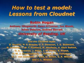
How to test a model:Lessons from Cloudnet Robin Hogan Anthony Illingworth, Ewan O’Connor, Jon Shonk, Julien Delanoe, Andrew Barratt University of Reading, UK And the Cloudnet team: D. Bouniol, M. E. Brooks, D. P. Donovan, J. D. Eastment, N. Gaussiat, J. W. F. Goddard, M. Haeffelin, H. Klein Baltink, O. A. Krasnov, J. Pelon, J.-M. Piriou, A. Protat, H. W. J. Russchenberg, A. Seifert, A. M. Tompkins, G.-J. van Zadelhoff, F. Vinit, U. Willen, D. R. Wilson and C. L. Wrench
Background • Clouds are very important for climate but poorly represented in models blah blah blah… • So what are we going to do about it? • Ways ARM-like observations can improve models: • Test model cloud fields (must be in NWP mode) • Test ideas in a cloud parameterization (e.g. overlap assumption, degree of inhomogeneity, phase relationship, size distribution) • But why is progress in improving models using these observations so slow? • Too many algorithmic/statistical problems to overcome? • Modelers and observationalists speak different languages? • Difficult to identify the source of a problem (dynamics, physics) when model clouds are wrong? • Comparisons too piecemeal: 1 case study, 1 model, 1 algorithm? • Climate modelers only interested in data on a long-lat grid? • NWP modelers need rapid feedback on model performance but usually papers published several years after the event?
Overview • The Cloudnet methodology • Evaluating cloud climatologies • Cloud fraction, ice water content, liquid water content • Evaluating the quality of particular forecasts • Skill scores, forecast “half-life” • Advantages of compositing • “Bony diagrams”, diurnal cycle • Improving specific parameterizations • Drizzle size distribution • Cloud overlap and inhomogeneity in a radiation scheme • Towards a “unified” variational retrieval scheme • How can we accelerate the process of converting observations into improved climate models?
The Cloudnet methodology • Project funded by the European Union 2001-2005 • Included observationalists and NWP modelers from UK, France, Germany, The Netherlands and Sweden • Aim: to retrieve and evaluate the crucial cloud variables in forecast and climate models • Seven models: 5 NWP and 2 regional climate models in NWP mode • Variables: cloud fraction, LWC, IWC, plus a number of others • Four sites across Europe (but also works on ARM data) • Period: Several years near-continuous data from each site • Crucial aspects • Common formats (including errors & data quality flags) allow all algorithms to be applied at all sites to evaluate all models • Evaluate for months and years: avoid unrepresentative case studies • Focus on algorithms that can be run almost all the time Illingworth et al. (BAMS 2007), www.cloud-net.org
Level 1b • Minimum instrument requirements at each site • Doppler cloud radar (35 or 94 GHz) • Cloud lidar or laser ceilometer • Microwave radiometer (LWC and to correct radar attenuation) • Rain gauge (to flag unreliable data) • NWP model or radiosonde: some algorithms require T, p, q, u, v
Liquid water path • Dealing with drifting dual-wavelength radiometers • Use lidar to determine whether clear sky or not • Optimally adjust calibration coefficients to get LWP=0 in clear skies • Provides much more accurate LWP in optically thin clouds LWP - initial LWP - lidar corrected Gaussiat, Hogan & Illingworth (JTECH 2007)
Level 1c • Instrument Synergy product • Instruments interpolated to the same grid • Calculate instrument errors and minimum detectable values • Radar attenuation corrected (gaseous and liquid-water) • Targets classified and data quality flag reported • Stored in one unified-format NetCDF file per day • Subsequent algorithms can run from this one input file
Level 1c • Instrument Synergy product • Example of target classification and data quality fields: Ice Liquid Rain Aerosol
Level 2a • Cloud products on observational grid • Includes both simple and complicated algorithms • Radar-lidar IWC (Donovan et al. 2000) is accurate but only works in the 10% of ice clouds detected by lidar • IWC from Z and T (Hogan et al. 2006) works almost all the time; comparison to radar-lidar method shows appreciable random error but low bias: use this to evaluate models
Level 2a • Liquid water content (+errors) on observational grid • “Scaled adiabatic” method (LWP +T + liquid cloud boundaries) Reflectivity contains sporadic drizzle: not well related to LWC LWC assumed constant or increasing with height has little effect on statistics
Cloud fraction Chilbolton Observations Met Office Mesoscale Model ECMWF Global Model Meteo-France ARPEGE Model KNMI RACMO Model Swedish RCA model
Statistics from AMF • Murgtal, Germany, 2007 • 140-day comparison with Met Office 12-km model • Dataset shortly to be released to the COPS community • Includes German DWD model at multiple resolutions and forecast lead times
Cloud fraction in 7 models • Uncertain above 7 km as must remove undetectable clouds in model • All models except DWD underestimate mid-level cloud • Some have separate “radiatively inactive” snow (ECMWF, DWD); Met Office has combined ice and snow but still underestimates cloud fraction • Wide range of low cloud amounts in models • Not enough overcast boxes, particularly in Met Office model • Mean & PDF for 2004 for Chilbolton, Paris and Cabauw 0-7 km Illingworth et al. (BAMS 2007)
A change to Meteo-France cloud scheme But human obs. indicate model now underestimates mean cloud-cover! Compensation of errors: overlap scheme changed from random to maximum-random • Compare cloud fraction to observations before & after April 2003 • Note that cloud fraction and water content entirely diagnostic beforeafter April 2003
Liquid water content • Met Office mesoscale tends to underestimate supercooled water • SMHI far too much liquid • ECMWF has far too great an occurrence of low LWC values • LWC from the scaled adiabatic method 0-3 km
Ice water content • ECMWF and Met Office within the observational errors at all heights • Encouraging: AMIP implied an error of a factor of 10! • IWC estimated from radar reflectivity and temperature • Rain events excluded from comparison due to mm-wave attenuation • For IWC above rain, use cm-wave radar (e.g. Hogan et al., JAMC, 2006) 3-7 km • Be careful in interpretation: mean IWC dominated by few large values; PDF more relevant for radiation • DWD has best PDF but worst mean!
How good is a cloud forecast? • So far the model climatology has been tested • What about individual forecasts? • Standard measure shows forecast “half-life” of ~8 days (left) • But virtually insensitive to clouds! ECMWF 500-hPa geopotential anomaly correlation • Good properties of a skill score for cloud forecasts: • Equitable: e.g. 0 for random forecast, 1 for perfect forecast • Proper: Does not encourage “hedging” (under-forecasting of event to get a better skill) • Small dependence on rate of occurrence of phenomenon (cloud)
Contingency tables Model cloud Model clear-sky Comparison with Met Office model over Chilbolton October 2003 Observed cloud Observed clear-sky
Simple skill score:Hit Rate • Misleading: fewer cloud events so “skill” is only in predicting clear skies • Models which underestimate cloud will do better than they should Met Office short range forecast • Hit Rate: fraction of forecasts correct = (A+D)/(A+B+C+D) • Consider all Cabauw data, 1-9 km • Increase in cloud fraction threshold causes apparent increase in skill Météo France old cloud scheme
More sophisticated scores • Yule’s Q =(-1)/(+1) where the odds ratio =AD/BC. • Advantage: little dependence on frequency of cloud • Equitable threat score =(A-E)/(A+B+C-E) where E removes those hits that occurred by chance. • Both scores are equitable: 1 = perfect forecast, 0 = random forecast • From now on use Equitable threat score with threshold of 0.05
Monthly skill versus time • Measure of the skill of forecasting cloud fraction>0.05 • Comparing models using similar forecast lead time • Compared with the persistence forecast (yesterday’s measurements) • Lower skill in summer convective events • Prognostic cloud variables: ECMWF, Met Office, KNMI RACMO, DWD • Entirely diagnostic schemes: Meteo-France, SMHI RCA
Skill versus lead time • Unsurprisingly UK model most accurate in UK, German model most accurate in Germany! • Half-life of cloud forecast ~2 days • More challenging test than 500-hPa geopotential (half-life ~8 days)
Cloud fraction “Bony diagrams” Winter (Oct-Mar) Summer (Apr-Sep) ECMWF model Chilbolton Cyclonic Anticyclonic
Cloud fraction “Bony diagrams” ECMWF overpredicts low cloud in winter but not in summer Winter (Oct-Mar) Summer (Apr-Sep) ECMWF model Chilbolton
Met Office mesoscale Observations Met Office global ECMWF Meteo-France KNMI RACMO SMHI RCA Andrew Barratt • 56 Stratocumulus days at Chilbolton
Drizzle • Radar and lidar used to derive drizzle rate below stratocumulus • Important for cloud lifetime in climate models O’Connor et al. (2005) • Met Office uses Marshall-Palmer distribution for all rain • Observations show that this tends to overestimate drop size in the lower rain rates • Most models (e.g. ECMWF) have no explicit raindrop size distribution
1-year comparison with models • ECMWF, Met Office and Meteo-France overestimate drizzle rate • Problem with auto-conversion and/or accretion rates? • Larger drops in model fall faster so too many reach surface rather than evaporating: drying effect on boundary layer? Met Office ECMWF model Observations
Ice water content from Chilbolton, log10(kg m–3) Plane-parallel approx: 2 regions in each layer, one clear and one cloudy “Tripleclouds”: 3 regions in each layer Agrees well with ICA when coded in a two-stream scheme Alternative to McICA Cloud structure in radiation schemes Height (km) Height (km) Height (km) Time (hours) Shonk and Hogan (JClim 2008 in press)
Vert/horiz structure from observations Horizontal structure from radar, aircraft and satellite: Fractional variance of water content 0.8±0.2 in GCM-sized gridboxes • CloudSat implies clouds are more maximally overlapped • But also includes precipitation (more upright?) CloudSat (Mace) • Vertical structure expressed in terms of overlap decorrelation height or pressure • Latitude dependence from ARM sites and Chilbolton Maximum overlap P0 = 244.6 – 2.328 φ TWP (MB02) SGP (MB02) Chilbolton (Hogan & Illingworth 2000) NSA (Mace & Benson 2002) Random overlap
Calculations on ERA-40 cloud fields Fixing just overlap would increase error, fixing just inhomogeneity would over-compensate error! SW overlap and inhomogeneity biases cancel in tropical convection Main LW effect of inhomogeneity in tropical convection Main SW effect of inhomogeneity in Sc regions TOA Shortwave CRF TOA Longwave CRF Long-wave CRF. Fix only inhomogeneity Tripleclouds (fix both) Plane-parallel Fix only overlap Tripleclouds minus plane-parallel (W m-2) …next step: apply Tripleclouds in Met Office climate model
Towards a “unified” retrieval scheme • Most retrievals use no more than two instruments • Alternative: a “unified” variational retrieval • Forward model all observations that are available • Rigorous treatment of errors • So far: radar/lidar/radiometer scheme for ice clouds • Fast lidar multiple-scattering forward model (Hogan 2006) • “Two-stream source function technique” for forward modeling infrared radiances (Toon et al. 1989) • Seamless retrieval between where 1 and 2 instruments see cloud • A-priori means retrieval tends back towards temperature-dependent relationships when only one instrument available • Works from ground and space: • Niamey: 94-GHz radar, micropulse lidar and SEVIRI radiometer • A-train: CloudSat radar, CALIPSO lidar and MODIS radiometer
Example from the AMF in Niamey 94-GHz radar reflectivity Forward model at final iteration 532-nm lidar backscatter 94-GHz radar reflectivity Observations 532-nm lidar backscatter
Results: radar+lidar only Large error where only one instrument detects the cloud Retrievals in regions where radar or lidar detects the cloud Retrieved visible extinction coefficient Retrieved effective radius Retrieval error in ln(extinction) Delanoe and Hogan (2008 JGR in press)
Results: radar, lidar, SEVERI radiances Cloud-top error greatly reduced TOA radiances increase retrieved optical depth and decrease particle size Retrieved visible extinction coefficient Retrieved effective radius Retrieval error in ln(extinction) Delanoe and Hogan (2008 JGR in press)
Lessons from Cloudnet • Easier to collaborate with NWP than climate modelers… • NWP models (or climate models in NWP mode) much easier to compare to single-site observations • Some NWP models are also climate models (e.g. Met Office “Unified Model”) so model improvements can feed into climate forecasts • Model evaluation best done centrally: it is not enough just to provide the retrievals and let each modeler test their own model • Feedback from NWP modelers: • A long continuous record is much better than short case studies: wouldn’t change the model based on only a month-long IOP at one site • Model comparisons would be much more useful if they reported in near-real-time (<1 month) because model versions move on so quickly! • Model evaluation is facilitated by unified data formats (NetCDF) • Observations: “Instrument Synergy” product performs most pre-processing: algorithm does not need to worry about the different instruments at different sites, or which pixels to apply algorithm to • Models: enables all models to be tested easily and uniformly
Suggestions… • A focus/working group on model evaluation? • To facilitate model evaluation by pushing “consensus” algorithms into infrastructure processing, and providing a framework by which models may be routinely evaluated • Include modelers, observationalists and infrastructure people • Devise new evaluation strategies and diagnostics • Tackle all the interesting statistical issues that arise • Promote ARM as a tough benchmark against which any half decent climate or NWP model should be tested • Need to agree on what a cloud is… • Probably not sensible to remove precipitating ice from observations: lidar shows a continuum between ice cloud and snow; no sharp change in radiative properties • By contrast, large difference between rain and liquid cloud
A global network for model evaluation • Build a framework to evaluate all models at all sites worldwide • Near-real-time processing stream for NWP models • Also a “consolidated stream” after full quality control & calibration • Flexibility to evaluate climate models and model re-runs on past data • 15+ sites worldwide: • ARM & NOAA sites: SGP, NSA, Darwin, Manus, Nauru, AMF, Eureka • Europe: Chilbolton (UK), Paris (FR), Cabauw (NL), Lindenberg (DE), New: Mace Head (IRL), Potenza (IT), Sodankyla (FI), Camborne (UK) • 12+ models to be evaluated: • Regional NWP: Met Office 12/4/1.5-km, German DWD 7/2.8-km • Global NWP: ECMWF, Met Office, Meteo-France, NCEP • Regional climate (NWP mode): Swedish SMHI RCA, Dutch RACMO • Global climate (NWP mode): GFDL, NCAR(via CAPT project)… • Embedded models: MMF, single-column models • Different model versions: change lead-time, physics and resolution • Via GEWEX-CAP (Cloud and Aerosol Profiling) Group?