Download
1 / 48
480 likes | 558 Views
Metalogical Properties of First Order Languages over Spatial Regions. Ernest Davis New York University Oct. 8, 2010 – CUNY Grad Center. Common belief about qualitative spatial reasoning. Languages for commonsense spatial reasoning should be: Qualitative

E N D
Metalogical Properties of First Order Languages over Spatial Regions Ernest Davis New York University Oct. 8, 2010 – CUNY Grad Center
Common belief about qualitative spatial reasoning Languages for commonsense spatial reasoning should be: • Qualitative • Refer to extended regions rather than points, lines, and other theoretical spatial constructs (Whitehead). Connected(p,q). Bigger(p,q). GOOD Dist(u,v) < 10.61. Curvature(c,p)=0.25. BAD • More plausible as a cognitive model (?) • More fundamental epistemologically (?) • More useful in applications, e.g. NLP (?) I don’t buy any of these, but these languages are interesting to study.
First-order spatial language One approach to qualitative spatial reasoning is to use a representation language that is: • First-order (Boolean operators, quantification over entities, equality) • The domain of entities is some collection of regions (assume topologically closed regular) • Limited vocabulary of relations • Language 1: Topological predicates • Language 2: Closer(x,y,z). • Language 3: C(x,y), Convex(x)
Examples • Define relations (non-recursive): C(x,y) ≝∿∃z Closer(x,z,y) P(x,y) ≡ ∀z C(z,x) ⇒ C(y,z) • Assert propositions ∀x,y P(x,y) ^ P(y,z) ⇒ P(x,z) ∀x∃y P(y,x) ^ y ≠ x What features can defined, and what propositions are true, depend on (a) what relations are in the language; (b) what is the domain of regions.
Not the Tarski language The Tarski language is the 1st order language of arithmetic over the reals. Can be used to implicitly quantify over a class of entities definable with a fixed number of real parameters. E.g. line in the plane (2 params), ellipse (5 params), dodecahedron (60 parameters). But not polygons in general, or regular regions.
Two kinds of results Elementary equivalence for topological language: Find a number of domains in which the same 1st order topological sentences are true. Expressivity of non-topological languages: In the first-order language with “Closer” or with “C” and “Convex” you can define practically any geometric property.
Outline of talk • Elementary equivalent domains. • Definitions and theorem statement • Non-examples • Lemma for proving elementary equivalence • Sketch of proof • Generalizations • Pratt-Hartmann’s theorem for planar collections • Expressivity of 1st order language • Theorem statements • Sketch of proof • Related Work • Open Problems
Topological relations Throughout, we will be working in k-dimensional, Euclidean space ℝk. A region is a subset of ℝk. Definition: A relation Γ(R1, …, Rk )is topological iff it is invariant under homeomorphisms of ℝkto itself. Examples. x ⊂ y. ∂x ⊂ y. x has a prime number of connected components. Non-examples: Dist(x,y)<3. x is a sphere.
Theorem Let R1 … Rm be topological relations over ℝk. Let L be a 1st-order language whose predicates correspond to R1 … Rm. Then the domain of rational polyhedra “Poly[ℚ]” in ℝk is elementary equivalent over L to the domain of polyhedra “Poly”.
Non-example 1 Fix a grid, and let Pixel be the set of all regions that are unions of grid squares. Then Pixel is not elementary equivalent to Poly, under any language in which “subset” can be defined. Proof: The sentence ∀x ∃y x ⊂y ^ x ≠ y is true in Poly but not Pixel.
Non-example 2 Let Rect be the collection of every region that is a finite union of aligned rectangles. Then Rect is not elementary equivalent to Poly for topological languages. Proof: The sentence, There exist 5 non-overlapping regions that meet at a point. is true in Poly but not in Rect.
Non-example 3. Let C be the collection containing all polyhedra and one solid disk. Let C1 be the Boolean closure of C. Then C1 is not elementary equivalent to Poly. Proof: The sentence For any regions A ⊊ B, there exists a region M such that A⊊ M⊊ B and ∂M⋂∂A = ∂M⋂∂B = ∂A ⋂∂B is true in Poly but not in C1.
Non-example 4 There are 2nd-order topological sentences that distinguish Poly from Poly[ℚ]. E.g. Any descending sequence R1 ⊃ R2⊃ R3 … of compact regions has a point in its intersection which is equal to A⋂B, for some regions A,B is true in Poly but not in Poly[ℚ].
A general method for proving elementary equivalence Let Ω be a set. Let 𝔸 be a group of bijections from Ω to Ω. Let B, C be subsets of Ω. Definition: B is finitely embeddable in C w.r.t𝔸 if for any b1, … bm in B there exists Γ in 𝔸 such that Γ(b1)… Γ(bm) are in C. Definition: B is extensible in C w.r.t. 𝔸 iff the following: For any b1 , … bm, bm+1 in B and Γ in 𝔸 such that Γ(b1)… Γ(bm) are in C, there exists Δ in 𝔸 such that Δ(b1)= Γ(b1) … Δ(bm)= Γ(bm) and Δ(bm+1) is in C.
Examples and non-examples of extensibility Let Ω=ℝ, the set of reals; B=ℚ, the set of rationals; C=ℤ, the set of integers. Let 𝔸 be the set of order-preserving homeomorphisms from ℝ to itself. B is embeddable in C w.r.t. 𝔸. C is not extensible in itself. If Γ(0)=0 and Γ(2)=1, then there is no possible value for Δ(1). Ω and B are mutually extensible.
Theorem of elementary equivalence Let R1 … Rm be relations over Ω that are invariant under 𝔸. Let L be a language with predicates R1 … Rm. Let B and C be subsets of Ω. If B and C are mutually extensible under 𝔸, then they are elementary equivalent under L. Example: ℚ and ℝ are elementary equivalent under the language with the predicate x<y.
Rectifiable mappings Let B be a subset of Ω. Let 𝔸 and 𝔾 be two groups of bijections of Ω to itself. 𝔸 is rectifiable to 𝔾 over B if the following holds: For any Γ in 𝔸 and b1 , … bmin B, if Γ(b1)… Γ(bm) are all in B, then there exists Δ in 𝔾 such thatΔ(b1)= Γ(b1) … Δ(bm)= Γ(bm).
Examples of rectifiable mappings Example: Ω= B=ℝ. 𝔸 is the set of order-preserving homeomorphisms over ℝ. 𝔾 is the set of order-preserving, piecewise-linear homemorphisms over ℝ. (Γ(x)=x3 is in 𝔸 but not in 𝔾.) Example: Ω= ℝ, B=ℚ . 𝔸 is as above. 𝔾 is the set of order-preserving, piecewise-linear, rational homeomorphisms.
Theorem Let C⊂B⊂Ω. Let 𝔸be a group of bijections from Ω to itself and let 𝔾 be a subgroup of 𝔸. If the following conditions hold: • B is closed under 𝔸. • C is closed under 𝔾. • B is embeddable in C under 𝔸. • 𝔸 is rectifiable to 𝔾 over C. Then B and C are mutually extensible w.r.t 𝔸.
Geometry B = Poly C = Poly[ℚ] 𝔸 = PL, the set of bounded piecewise-linear homemorphisms fromℝk to itself. 𝔾 = PL[ℚ], the set of bounded piecewise-linear rational homemorphisms fromℝk to itself. To prove: B is embeddable into C under 𝔸. 𝔸 is rectifiable to 𝔾 over C.
Piecewise linear mapping a = <0,0> a’=<2+ √(10/19), 0> b = <1/√2> b’=<3,0> c = <1,0> c’=<3, √(11/23)> d=<1/√3, 1-1/√3> d’=<3,1> e=<1/√5, 1-1/√5> e’= <2+√(14/29),1> f=<1/ √7, 1-1/ √7> f`=<2,1> g=<0,1> g’=<2,√(15/31)> h=<0, 1/√11> h’=<2,0> i=<2/3, √ (2/3) I’=< √(3/4), 3/4>
General idea of proof We’re going to slide each of the points on both sides to a nearby rational point that stays on the same side of the triangle. To prove: This can be done without messing up the topology.
Simplices and Complexes: Definitions An abstract simplex is a set of vertex names. E.g. {a, h, i}. An abstract complex is a collection of simplices, closed under subset. E.g. {{a,b,c}, {a,b,d}, {a,b}, {a,c}, {a,d}, {b,c}, {b,d},{a}, {b}, {c}, {d}, {} }
Instantiations An instantiation is a mapping over vertex names to points in ℝk. Thus, an instantiation can be viewed as a point in ℝkz , z=number of vertices. An instantiation associates an abstract simplex S with the geometric simplex, Hull(Γ(S)) It associates the abstract complex C with the geometric complex { Hull(Γ(S)) |S ∈ C }
Respectful Instantiations Let C be a complex and let Γ be an instantiation. Γ respects C if: • Γ maps each simplex S in C to an affine independent set. E.g. if |S|= 3, then Γ(S) is not collinear. If |S|=4, then Γ(S)is not coplanar. • If S,T are in C, then Hull(Γ(S))⋂Hull(Γ(T)) = Hull(Γ(S⋂T)). Γ(C) is a triangulation of |Γ(C)|
Example: C={{a,b,c}, {a,b,d}, {a,b}, {a,c}, {a,d}, {b,c}, {b,d},{a}, {b}, {c}, {d}, {} }
Lemmas The set of rational instantiations is dense in the space of instantiations. The set of instantiations that respect C is open in the space of instantiations. Therefore given any instantiation that respects C, there exists a nearby rational instantiation that respects C.
Rectifying a PL mapping to a rational PL mapping Given • P1, …, Pm ∈ Poly[ℚ ] • Bounded PL mapping Γs.t. Γ(P1), …, Γ(Pm ) ∈ Poly[ℚ ] Construct a big rational box B s.t. Γ is the identity outside B. Let U1 … Uq be the intersections of B, P1, …, Pm with the cells of Γ’. Let T be a triangulation of {U1 … Uq}. Γ’(T) is a triangulation of {Γ’(U1) … Γ’(Uq)}. Move every vertex of T and of Γ’(T) to a nearby rational point on the same face of B, P1, …, Pm Let Δ be the PL-mapping moving each new location of vertex v in T to the new location of Γ’(v) . Extend Δ to interior points using barycentric coordinates.
Generalizations • Can use Poly[𝔽] where 𝔽 is any subfield of ℝ. • Can extend to unbounded polytopes. (Use piecewise projective transformation to map to bounded polytopes.) • Can extend to o-minimal collections (e.g. semi-algebraic regions). (Proof by Googling; all the heavy lifting was done by Tarski, van den Dries, and Shiota).
Planar collections (Ian Pratt-Hartmann) Let C be a collection of regions in the plane with the following properties: • Closed under union, regularized intersection, regularized set difference. • For every open set O, for every point p in O, there exists R in C such that p ∈ R ⊂ O. • Every region has finitely many connected components. • If R ∈ C and u and v are identifiable points on ∂R, then R=R1⋃ R2 where R1, R2 ∈ C and R1 ⋂ R2 is a simple curve from u to v. • If R ∈ C and u is an identifiable point on ∂R, then there is a curve starting at u and otherwise in interior(R). Then C is elementary equivalent to Poly under any topological language.
Example Let C be the Boolean closure of all rectangles and all circular disks. Then C satisfies Pratt-Hartmann’s conditions and therefore is elementary equivalent to Poly for any topological language. Note: This theorem has only been proven for the plane.
Expressivity Consider the 1st-order language with predicate “Closer’’ C(x,y) ¬∃(z) Closer(x,z,y) P(x,y) ∀(z) C(z,x) → C(z,y) Universe of regions: Any collection of closed regions that contains all simple polygons.
Question: What properties can be expressed in this representation? Answer: Just about anything • X and Y have the same area. • X and Y are homeomorphic. • X is an L by W rectangle where L/W is a transcendental number. • X is the graph of a Bessel function* • X is a polygon with N sides where N is the index of a non-halting Turing machine • The boundary of X has fractal dimension 1.5.* * Assuming the universe contains these.
What can’t be represented? 1. Properties that are not invariant under orthogonal transformation: “X is 1 foot away from Y” “X is due north of Y” 2. Distinguishing between two sets with the same closure. 3. Properties of remote logical complexity “The number of connected components of X is in set S”, where S⊂ℤ cannot be represented by any 2-order formula.
Analytical relations Let ω be the set of integers, and let ωω be the set of infinite sequences of integers. Let U= ω∪ωω. A relation over UI is analytical if it is definable as a first-order formula using the functions +, *, and s[i] (indexing). (2nd order arithmetic)
Other analytical structures Lemma: The real numbers ℝ with functions + and * and predicate Integer(x) is mutually definable with UI. (Contrast: ℝwith + and * is decidable. ℕwith + and * is first-order arithmetic.) Lemma: The domain ℝ∪ ℝωis mutually definable with UI.
Analytical relations over regions Observation: A closed region is the closure of a countable collection of points. Definition: Let C be a coordinate system, and let Φ(R1 … Rk) be a relation on regions. Φ is analytical w.r.t. C if the corresponding relation on the coordinates of sequences of points whose closure satisfy Φ is analytical.
Theorems Theorem: Let U be a class of closed regions that includes all simple polygons. Let Φ be an analytical relation over U. • If Φ is invariant under orthogonal transformations, then it is definable in a first-order formula over “Closer(x,y,z)”. • If Φ is invariant under affine transformations, then it is definable in terms of “C(x,y)” and “Convex(x)”.
Steps of Proof • Define a point P as a pair of regions that meet only at P. • Define a coordinate system as a triple of points (origin, <1,0>, and <0,1>). • Define a real number as a point on a coordinate system. • Define +, *, and Integer(x) on real numbers. • Define coords(P,C,X,Y).
Real Arithmetic Addition Multiplication
Integer length S is connected, and for every point P in S, there exists a horizontal translation v such that P ∈ T+v⊂S and U+v is outside S.
Expressing a relation Φon regions • Construct a relation Γ(p1,1, p1,2, … p2,1, p2,2, … pk,1,pk,2…) which holds if and only if Φ(Closure(p1,1, p1,2, …), Closure(p2,1, p2,2, …) … Closure(pk,1, pk,2, …) ) 2. Translate Γ into a relation on the coordinates of the p’s. 3. Express in terms of Plus, Times, Integer
Related Work • (Grzegorczyk, 1951). The first-order language with C(x,y) is undecidable. • (Cohn, Gotts, etc. 1990’s) Work on expressing various relations in various 1st order languages. • (Pratt and Schoop, 2000) Let P1 … Pk be a tuple of polygons in ℝ2 or ℝ3. The relation over R1 … Rk, ``There is a homeomorphism mapping all the Ri to Pi’’ is expressible in the 1st order language of C(x,y). • (Schaefer and Stefanovich, 2004) The first-order language with C(x,y) has analytical complexity (not expressivity). • Lots of work on constraint (existential) languages.
Open Problems Find geometric conditions (similar to Pratt-Hartmann’s) for elementary equivalence to Poly in ℝk for k > 2. What is the expressivity of the first-order language with just C(x,y)? Analogue: If Φ is analytical and topological then it can be represented.
Definition of Point AllCloser(a,b,c) ∀z C(z,b) → Closer(a,z,c) InInterior(a,b) ∃d ¬C(d,a) ^ ∀c AllCloser(a,c,d) → P(c,b). Regular(b) ∀c,d C(c,b) ^ ¬C(c,d) → ∃a Closer(c,a,d) ^ InInterior(a,b).
Definition of Point (cntd) IsPoint(a,b) Regular(a) ^ Regular(b) ^ ∀c,d [P(c,a) ^ P(d,b) ^ C(b,c) ^ C(d,a)] → C(c,d) SamePoint(a,b,c,d) IsPoint(a,b) ^ IsPoint(c,d) ^ ∀w,x,y,z [P(w,a) ^ P(x,b) ^ P(y,c) ^ P(z,d) ^ C(w,x) ^ C(y,z)] → C(w,y)
Properties of Points InPt(a,b;r) ∀d,c SamePoint(d,c;a,b) → C(d,r). PtCloser(p,q,r) ∀a,b,c Regular(a) ^ Regular(b) ^ Regular(c) ^ InPt(p,a) ^ InPt(q,b) ^ InPt(r,c) → ∃d,e,f P(d,a) ^ P(e,b) ^ P(f,d) ^ Closer(d,e,f).