Download
1 / 25
250 likes | 339 Views
Explore the proposed algorithm for minimizing redundant transmissions in single-message broadcasts within 2-D distributed networks. Understand the advantages and challenges of flooding in comparison to the proposed algorithm. Learn about local broadcast algorithms, static and dynamic approaches, and the responsibility condition for efficient information dissemination.

E N D
Broadcasting with Bounded Number of Redundant Transmissions Majid Khabbazian
Outline • Assumptions • Objectives • Classifications • The proposed algorithm • Algorithm’s characteristics • Conclusion
Assumptions • Single message broadcast • Nodes are distributed in 2-D space • The transmission range of each node is R • We can use Unit Disk Graph (UDG) to model the network • No Synchronization • Perfect Medium Access Control (MAC) • No errors or collisions • Neighbors don’t transmit at the same time • Nodes are static during the broadcast
Objectives • End-to-end delay is NOT a concern • What do we care about? • Full delivery • Reducing the number of transmissions • Each node has a local view of the network
Flooding: A Simple Solution • Flooding • Every node transmits the first copy of received message • Pros. • A simple solution • No need to have neighbor information • Requires almost no computation • Cons. • All the nodes transmit the message • It can cause a large number of redundant transmissions • It can lead to significant performance degradation and network congestion
A Question • Can we minimize the total number of transmissions? • This is related to fining a Minimum Connected Dominating Set (MCDS) • Finding MCDS is NP-hard even for UDGs • Good approximation algorithms? • Case 1: The whole topology is known • Case 2: Each node has a local view of the network • Local Broadcast Algorithms
Local Broadcast Algorithms • Classifications • Static (Proactive) • Dynamic (Reactive) • Static Approach • A backbone is constructed first • The backbone is a Connected Dominating Set • Pros. • Can be used for both broadcasting and unicasting • Cons. • May not be good where the network topology is dynamic • The backbone is fixed in the static network
Local Broadcast Algorithms (Con’d) • Dynamic Approach • There is no backbone • Nodes decide “on-the-fly” based on their local view • Pros. • The backbone changes from one network-wide broadcast to another (even for the single source) • More robust against failures than static approach • Cons. • Constructed backbone may not be stable
Further Assumptions • Each node has the list of its 1-hop neighbors • Exchanging “hello” messages • Geographical information is available • E.g., Using GPS • Relative distance may suffice
Static Approach • A small size backbone can be easily constructed • Regionalizing the network • Selecting a constant number of nodes in each region • Example: • Divide the network into square cells with diameter 1 • At most 20 nodes have to be selected in each cell
Dynamic Approach • Can we reduce the total number of transmissions in the worst case? • Is constant approximation factor achievable? • Our proposed algorithm is proven to achieve: • Full delivery • Constant approximation factor
Proposed Algorithm • Each node decides on its own whether or not to transmit • Before transmitting, the node removes the information attached to the message and adds the list of its 1-hop neighbors to the message • The decision is made based on a self-pruning condition called the responsibility condition • The closer, the more responsible
Responsibility Condition • A node u has to transmit the message if it has a neighbor v s.t. • v has not received the message AND • There is no node w such that w has received the message and dist(wv )< dist(uv)
Example • A receives the message from H • A knows that E, F and G have received the message and B, C and D have not • Based on the responsibility condition A does not need to transmit the message G D F C H A B E
Full Delivery • It achieves full delivery • Proof by contradiction: • The broadcast will eventually terminate • Suppose there is a node that has not received the message • Consider the set • S={(u,v)| u and v are neighbors, u has received the message, v has not received the message} • S is not empty
Full Delivery (Con’d) • S is not empty There exists a pair (u’,v’) in S such that Dist(u’,v’)<= dist(u,v) for any pair (u,v) in S. • u’ has the highest responsibility toward v’ • v’ has not receive the message • Based on the responsibility condition • u’ must have transmitted the message
Approximation Factor • The proposed algorithm achieves a constant approximation factor Sketch of proof • There are at most a constant number of transmissions in each disk with radius ¼ • Transmission coverage of each node is a disk with radius 1 • Each node has a constant number of neighbors that transmit the message • The number of transmission has to be within a constant factor of the optimum
Approximation Factor (Con’d) • Transmitters: Blue nodes • Blue nodes are neighbors • All the nodes in the white disk will get the message after the first transmission • Blue nodes are aware of this fact
Approximation Factor (Con’d) • Every blue node is responsible for a unique red node • The distance between a blue and a red node is at least ½ • The number of red nods must be constant
Relaxing Some of the Assumptions • Similar results can also be achieved when • Nodes are distributed in 3-dimensional space • Nodes can have different transmission ranges • Nodes don’t have IDs • Geographical information is not accurate • Error must be less than ~0.1 • Geographical information can be represented using a constant number of bits • Key Idea: Each node required to report its position to its neighbors
Simulation • We compared the performance of the proposed algorithm with • Liu’s algorithm [Infocom 2006 ] • A ratio-8 approximation algorithm [Infocom 2002 ] • Used as a benchmark
Example • #nodes: 400 • Trans. range: 300meter • #broadcasting nodes: 10
Conclusion • Reactive broadcast algorithms are in fact powerful • Question: Can we do this without using geographical info. (or relative distances)? • The answer is YES. This can be the subject of a future talk..