Download

1 / 1
10 likes | 162 Views
GH-3. GH-2. GH-1. Figure 1. Illustrates the key differences between sheet and concentrated flows for controlling overland flow transport. Unless proper management practices are implemented, permanent gully erosion may develop. The Effects of Different Resolution DEMs

E N D
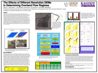
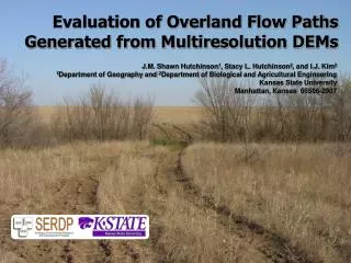
GH-3 • GH-2 • GH-1 Figure 1. Illustrates the key differences between sheet and concentrated flows for controlling overland flow transport. Unless proper management practices are implemented, permanent gully erosion may develop. The Effects of Different Resolution DEMs in Determining Overland Flow Regimes Stacy L. Hutchinson1, J.M. Shawn Hutchinson2, Ik-Jae Kim1,and Philip Woodford31Department of Biological and Agricultural Engineering and 2Department of Geography, Kansas State University, Manhattan, Kansas 3Integrated Training Area Management, Fort Riley, Kansas Abstract A gully head is a unique landscape feature where concentrated overland flow begins to cause significant erosion. The impacts of four different resolution digital elevation models (DEMs), three (3, 10, and 30 m) developed using a differential global positioning system (GPS) survey and the USGS 30 m DEM, were used to identify transitional flow areas on a grassland hillslope. A simple erosion model, nLS, based on Manning’s kinematic wave theory, was used to determine where overland flow transitioned from sheet flow to concentrated flow. The accumulated erosive energy was estimated using the nLS model, where, n is Manning’s coefficient, L is the overland flow length, and S is the slope. In addition to the DEMs, spatial analyses for soil (SSURGO) and land cover (Kansas GAP) were conducted in a geographic information system (GIS). First order streams were delineated using each resolution DEM (contributing area: 900 m2) and overlaid with the concentrated flow data obtained from the nLS model results. The intersected area was buffered by 3, 6, 10, or 15 m, depending on the DEM resolution. Results showed that average topographic and hydrologic variables varied between the different DEM resolutions. The 3 m DEM produced the best model accuracy, predicting two gully head locations. The recommended buffer radius was found to be 6 m, which is 2 times of the grid size. The efforts to develop finer data resolution should be supported in assessing reliable erosion potential for watershed management. Figure 4. RMSE of random sample points (5 %) for different resolution DEMs using IDW and TIN interpolation methods. Results show that 10 m DEMs offer more reliable prediction for hydrologic modeling than 30 m DEMs. However, the errors in 10 m DEMs were 2.44 (IDW) or 2.55 (TIN) times greater than in 3 m DEMs. No difference was seen between interpolation techniques. Figure 2. The study site, 8 ha grass-hillslope area on Fort Riley with GPS points (n > 15,000) and three gully head locations (red). Two areas on the upslope and one at the downslope were excluded from the survey to avoid field experiments and dense vegetation. Three gully locations (GH-1, 2, and 3) were surveyed. Concentrated Flow A = W x L x β β = A – Ineffective Area Uniform Sheet Flow A = W x L L W Figure 5. Accumulated overland flow energy calculated using nLS with different resolution DEMs (left). Potential erosion areas based on 1st order stream networks and acumulated overland flow energy (μ±1.0σ of nLS) with buffering using different resolution DEMs (right). A gully erosion area (GH-3) on the study site in figure 2. (Taken on Oct. 15, 2005 by IJ Kim) Data and Methods Three different resolution (3, 10, and 30 m) digital elevation models (DEMs) were developed using a differential GPS with post-processing. Two interpolation techniques (inverse distance weighted, (IDW) and triangulated irregular network, (TIN)) were used for converting from GPS point data to raster format files for each resolution. The vertical and horizontal errors were assessed using root mean square error (RMSE) on 5 % randomly selected points and two benchmarks. The USGS National Elevation Dataset (NED) 30m DEM was also used to develop accumulated erosive energy layers within ESRI ArcGIS using the nLS model. Input variables (slope and flow length) were calculated using the deterministic eight direction method (D8). Flow direction was estimated without the ‘pit’ removal process. This artificial process may alter the effect of accumulating overland flow energy for identifying the flow transition from sheet to concentrated flow. Flow length for each cell was determined by multiplying the flow accumulation values by the DEM resolution. Kansas GAP landcover data were used to create Manning’s coefficient (n) data layers. From the information, a continuous “energy accumulation” grid was developed using the equation (1). The statistical interval (μ±1.0σ, in English Unit) of mean (μ, 131) and standard deviation (σ, 22.6) was applied to reclassify the transitional areas (i.e., gully head locations). It was assumed that gully heads are formed along the 1st order streams. The selected 1st order stream segments were buffered, using 3 m and 6 m (in radius) for the 3 m DEMs, 10 m for the 10 m DEMs, and 15 m for the 30 m DEMs to account for data resolution errors in identifying gully head points. Conclusions and Future Work Finer resolution DEMs provided more detailed land analysis than coarser resolution DEMs. Accurate slope estimation was very important in this study because the lengths of gully head from the upslope are generally less than the lengths of the hillslope. Errors in slope estimates significantly affected the model performance when generating the flow direction and flow accumulation grids. Current results suggest that 3 m or finer DEMs should be used to determine the geographic locations of gully heads in the model. Further analysis using a large area and or complete watershed is needed to investigate the impact of study area size and different land covers. The influence of the ‘pit’ removal process should be evaluated. Additionally, the effect of varying contributing areas for delineating the 1st order stream network using the same fine resolution DEM should be analyzed. Key references McCuen, R.H. and J.M. Spiess. 1995. Assessment of kinematic wave time of concentration. Journal of Hydrologic Engineering 121 (3):256-266. Meyer, A. and J.A. Martinez-Casasnovas. 1999. Prediction of existing gully erosion in vineyard parcels of the NE Spain: a logistic modeling approach. Soil & Tillage Research 50: 319-331. Acknowledgements This work is funded through CPSON-03-02 (Characterizing and Monitoring Non-Point Source Runoff from Military Ranges and Identifying their Impacts to Receiving Water Bodies). Figure 3. A methods data flow diagram for determining transitional erosion areas in a GIS. (C.A. means the contributing area for delineating 1st order stream networks using the flow accumulation grids). Table 1. Root mean square errors (RMSE) for the GPS survey at the two temporary benchmark points (BM1: east and BM2: west in figure 2). Equation (1) • n: Manning’s coefficient • L: Flow length (m) • S: Slope (m/m)