Download
1 / 37
370 likes | 521 Views
QoS Routing Using Traffic Forecast - A Case Study of Time-Dependent Routing. Yuekang Yang Chung-Horng Lung Dept. of Systems and Computer Engineering, Carleton University. Scope. Assumes that aggregated Internet traffic has a periodic predictable pattern

E N D
QoS Routing Using Traffic Forecast- A Case Study of Time-Dependent Routing Yuekang Yang Chung-Horng Lung Dept. of Systems and Computer Engineering, Carleton University
Scope • Assumes that aggregated Internet traffic has a periodic predictable pattern • Only the link capacity constraint and QoS constraints are considered in the discussion • Link or node failure and traffic backup are not considered in this research • Intra-domain QoS routing SCE, Carleton University
Outline • Introduction • Methodology • Simulation Results of the State-Dependent Routing Mechanism • Simulation Results of the Time-Dependent Routing Mechanism • Conclusions SCE, Carleton University
QoS Routing • QoS Routing is a part of Constraint-Based Routing • CBR denotes a class of routing algorithms that base path selection on a set of constraints, in addition to the destination. • If constraints imposed are QoS requirements, the associated routing is referred to as QoS routing. • Other constraints in CBR could be administrative policies. • Constraints in QoS Routing • Bandwidth • Delay • Packet loss SCE, Carleton University
Challenges of QoS Routing • Stability and Scalability • When multiple resources are allocated and deallocated, high frequency of state updates is required to avoid instability and route flapping, but it does not scale well due to its high communication overhead for large networks. • Robustness • Routers always get state updates with delays, and there is no guarantee that resource information is accurate and up-to-date. Route computation and routing decisions should be robust enough based on imprecise states. • Routing Cost • Processing state updates, implementing techniques related to robustness issue, and conducting QoS routing (an NP-Complete problem) introduce considerable computational cost. Contrastively, QoS requests expect highly responsive services. SCE, Carleton University
Research Motivation Adapted from: “Long-Term Forecasting of Internet Backbone Traffic - Observations and Initial Models,” Proc. Conf. Comp. Commun., IEEE INFOCOM, March 2003. SCE, Carleton University
QoS Routing Using Traffic Forecast • State-Dependent/Time-Dependent Mechanism • A routing algorithm that is able to find the optimal route for every QoS request, without knowing either the history or the future traffic demand, is called state-dependent mechanism. • A routing algorithm that has knowledge of the history or future traffic demand is called time-dependent mechanism. • Three Questions Addressed in This Research • Can traffic forecasting improve QoS routing performance? • What if the forecast is not perfect? • What kind of traffic forecast is required for QoS routing? SCE, Carleton University
Outline • Introduction • Methodology • Simulation Results of the State-Dependent Routing Mechanism • Simulation Results of the Time-Dependent Routing Mechanism • Conclusions SCE, Carleton University
Simplification on QoS Constraints • Delay and loss • Latency formula from the hypothesis that each queue behaves as an M/M/1 queue of packets: • De is the processing and propagation delay on edge e, and ce is the link capacity of edge e. Both De and ce could be considered as constant. xe is the total bandwidth required for all flows on edge e. • It shows that new assigned QoS request can affect the delay of old flows. • So the upper bounds of delay and loss for each edge are adopted to simplify the QoS routing problem in this work. It is justified by the fact that the measured loss probabilities and delay for the same QoS on different routers are of similar order. Hence, the number of hops along a route is considered as the constraint. • Bandwidth • Equivalent bandwidth is calculated according to burstiness, buffer size, flow peak/link ratio. SCE, Carleton University
Objectives in QoS Routing • Two major objectives in QoS Routing • Provide routing service with overall low network resource consumption. In other words, minimize the average number of hops that those routes traverse. • Avoid overloading parts of the network while other parts are under-loaded. That is to minimize the maximum link utilizations. There are three reasons: • Spare bandwidth is available at various parts of the network to accommodate unpredictable traffic requests. • In case of link failures, smaller amounts of traffic will be disrupted and will need to be rerouted. • Nodal router performance, such as delay, degrades dramatically when router’s load approximates its maximum capacity. • In most cases, these objectives are not conformable with each other SCE, Carleton University
Performance Evaluation • The Objective Function in Optimization • ce is the link capacity on edge e. xe,k is the bandwidth of the kth flow on edge e. K represents the set of all flows in a network. • The order n is a useful tool for ISPs to get more accurate results • Based on this objective function, the optimal solution of routing can be calculated by the general gradient projection method. • The value of this objective function can also be seen as an performance metric when different routing algorithms are compared. SCE, Carleton University
Outline • Introduction • Methodology • Simulation Results of the State-Dependent Routing Mechanism • Simulation Results of the Time-Dependent Routing Mechanism • Conclusions SCE, Carleton University
Simulation Setup- Network #1 SCE, Carleton University
Simulation Setup- Network #2 SCE, Carleton University
Simulation Results- Network #1 SP: shortest path WSP: widest shortest path SWP: shortest widest path SCE, Carleton University
Simulation Results- Network #2 SCE, Carleton University
Analysis of State-Dependent Mechanism • Underlying Problems with State-Dependent Mechanism • State-dependent mechanism faces all challenges mentioned before, no matter it is designed as Pre-Computation Routing or On-Demand Routing. In particular, pre-computing paths for all possible QoS requirements is extremely processor and memory consuming, as it has no idea about the future demands. • Rearrangement dilemma • To avoid rearrangement as much as possible, the performance of state-dependent routing algorithms degrades gradually as the traffic demand increases. • It is difficult for state-dependent routing algorithms to reach performance optimal points when the traffic demand is at a moderate level. SCE, Carleton University
Rearrangement Dilemma • Some flows have to be rearranged in terms of explicit routes and their assigned bandwidth. Rearrangement causes service disruption and significant signaling overhead to proceed with minimal disruption. The cost of rearrangement increases dramatically as rearrangement becomes frequent. • Suppose a state-dependent mechanism can approximate an optimal point according to the current state. After a few minutes when new LSP requests come in, it has a high chance to rearrange existing user flows in order to keep the same level of performance. On the other hand, if fewer rearrangements are needed, it has to stay away from the optimal points. The dilemma partially stems from the ignorance of future traffic demand. SCE, Carleton University
Outline • Introduction • Methodology • Simulation Results of the State-Dependent Routing Mechanism • Simulation Results of the Time-Dependent Routing Mechanism • Conclusions SCE, Carleton University
Design a Time-Dependent RoutingAlgorithm • For a request of bandwidth bw from source node s to destination node d, with hop count constraint c, the pseudo code for the TDWSP is as follows: initialize expectedBw, plannedFreeBw, residueFreeBw if bw < expectedBw(s,d) { do WSP(s,d,c) on plannedTree if success { expectedBw(s,d) = expectedBw(s,d) - bw plannedFreeBw(s,d) = plannedFreeBw(s,d)- bw } else { do WSP(s,d,c) on residueNet if success { residueFreeBw(s,d) = residueFreeBw(s,d)- bw } } } else { do WSP(s,d,c) on residueNet if success { residueFreeBw(s,d) = residueFreeBw(s,d)- bw } } SCE, Carleton University
Traffic Demands SCE, Carleton University
Simulation ResultsNetwork #2, the first line of traffic demands WSP: widest shortest path TDWSP: time-dependent widest shortest path SCE, Carleton University
Simulation ResultsNetwork #2, the second line of traffic demands SCE, Carleton University
Simulation ResultsNetwork #2, the third line of traffic demands SCE, Carleton University
Advantages of the Time-Dependent Mechanism • Now the challenges mentioned in the beginning of the presentation are reexamined in the context of time-dependent mechanism. • For most LSP requests that the TDWSP expects, ingress router can make routing decision just based on preplannedlocal information. Only when unexpected requests come in, TDWSP uses WSP algorithm on the residue network. The existence of this fast execution path can mitigate all those challenges we discussed before. • TDWSP has a lower standard deviation for the objective function value than WSP when the traffic load is below the level forecasted. In other words, TDWSP is less sensitive to the order of QoS requests than WSP. • The modification from WSP to TDWSP could facilitate a distributed implementation. SCE, Carleton University
Analysis of the Time-Dependent Mechanism • When the offered traffic load is not heavy in terms of the maximum traffic a network can handle, a time-dependent variation of the state-dependent routing algorithm could perform very close to the optimal boundary. • When the offered traffic load is heavy, the performance of a time-dependent routing algorithm is degraded. • If the demand forecast is at the moderate traffic level, a time-dependent routing algorithm could be insensitive to the position of the forecast. One fixed forecast may be effective enough to optimize the routing performance in a large area. SCE, Carleton University
Outline • Introduction • Methodology • Simulation Results of the State-Dependent Routing Mechanism • Simulation Results of the Time-Dependent Routing Mechanism • Conclusions SCE, Carleton University
Conclusions • The inherent disadvantages of state-dependent mechanisms, due to the lack of prediction of traffic. In order to avoid rearrangement to support QoS routing, the performance of SP, WSP and SWP is not optimized when the traffic load grows. • The benefits of traffic forecasting in the time-dependent mechanism are further explained in light of its positive impact on routing performance. • TDWSP outperforms WSP under almost all traffic conditions in both networks, #1 and #2. TDWSP greatly relaxes the burden of QoS database synchronization among routers, and hence eases the challenges of scalability, robustness and routing cost. SCE, Carleton University
Backup slides SCE, Carleton University
The Curvature of the Objective Function • The objective function is: • This objective function is a sum of link costs. • The diagram shows the link cost increases with the link utilization. SCE, Carleton University
Effect of the Curvature of the Objective Function SCE, Carleton University
Effect of the Curvature of the Objective Function SCE, Carleton University
Simulation ResultsNetwork #1, the first line of traffic demands SCE, Carleton University
Simulation ResultsNetwork #1, the second line of traffic demands SCE, Carleton University
Simulation ResultsNetwork #1, the third line of traffic demands SCE, Carleton University
The Solvable Traffic Demand Space • For instance, a four-node network has the following traffic matrix: • The traffic matrix can also be represented in vector form when the topology information is not relevant to the discussion. • Imagine a space that consists of the end-points of all legitimate vector d, and call it the traffic demand space. • From the routing point of view, in this research we define a solvable traffic demand space as a subset of the traffic demand space with at least one feasible routing solution, no matter whether the feasible routing solution is optimized or not. SCE, Carleton University
Implications • The unsymmetrical insensitivity of the traffic demand does suggest that the extreme value of the daily traffic orbit might be the focus of the traffic forecast. If the routing performance under peak traffic is good, then the routing performance during the rest of the day should be fine. • The size and shape of the solvable traffic demand space is determined if the topology of a network has been finalized. However, the solvable traffic demand space is not very large, given a topology. The mapping from the solvable space to specific routing solutions is the job of the QoS routing algorithms. If our focus is turned toward the solvable space that is not large in size, then it seems reasonable to introduce the time-dependent routing mechanism. SCE, Carleton University