Download
1 / 75
780 likes | 1.3k Views
Analysis of Convection Heat Transfer. P M V Subbarao Professor Mechanical Engineering Department IIT Delhi. Development of Design Rules …. Methods to evaluate convection heat transfer. Empirical (experimental) analysis

E N D
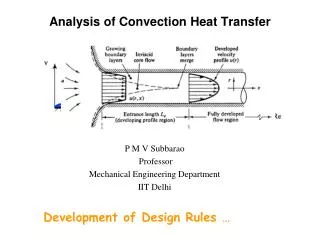
Analysis of Convection Heat Transfer P M V Subbarao Professor Mechanical Engineering Department IIT Delhi Development of Design Rules …
Methods to evaluate convection heat transfer • Empirical (experimental) analysis • Use experimental measurements in a controlled lab setting to correlate heat and/or mass transfer in terms of the appropriate non-dimensional parameters • Theoretical or Analytical approach • Solving of the energy equations for a particular geometry. • Example: • Solve for q • Use evaluate the local Nusselt number, Nux • Compute local convection coefficient, hx • Use these (integrate) to determine the average convection coefficient over the entire surface • Exact solutions possible for simple cases. • Approximate solutions are also possible using an integral method
Empirical method • How to set up an experimental test? • Let’s say you want to know the heat transfer rate of an airplane wing (with fuel inside) flying at steady conditions…………. • What are the parameters involved? • Velocity, –wing length, • Prandtl number, –viscosity, • Nusselt number, • Which of these can we control easily? • Looking for the relation:Experience has shown the following relation works well:
L insulation Experimental test setup • Measure current (hence heat transfer) with various fluids and test conditions for • Fluid properties are typically evaluated at the mean film temperature
Theoretical or Analytical approachSolving of the boundary layer equations for a particular geometry.
Internal Flows • Internal flow can be described as a flow whose boundary layer is eventually constrained as it develops along an adjacent surface. • The objectives are to determine if: • the flow is fully developed (no variation in the direction of the flow • laminar or turbulent conditions • the heat transfer
Temperature Profile in Internal Flow Hot Wall & Cold Fluid q’’ Ts(x) Ti Cold Wall & Hot Fluid q’’ Ti Ts(x)
External Flows • Any property of flow can have a maximum difference of Solid and free stream properties. • There will be continuous growth of Solid surface affected region in Main stream direction. • The extent of this region is very very small when compared to the entire flow domain. • Free stream flow and thermal properties exit during the entire flow. T T T T T T
1904 A continuously Growing Solid affected Region. The Boundary Layer Ludwig Prandtl
1822 1752 1860 1904 De Alembert to Prandtl Ideal to Real
Introduction • A boundary layer is a thin region in the fluid adjacent to a surface where velocity, temperature and/or concentration gradients normal to the surface are significant. • Typically, the flow is predominantly in one direction. • As the fluid moves over a surface, a velocity gradient is present in a region known as the velocity boundary layer, δ(x). • Likewise, a temperature gradient forms (T ∞ ≠ Ts) in the thermal boundary layer, δt(x), • Flat Plate Boundary Layer is an hypothetical standard for initiation of basic analysis.
Velocity Boundary Layer d(x) Fluid particles in contact with the surface have zero velocity u(y=0) = 0; no-slip boundary condition Fluid particles in adjoining layers are retarded δ(x): velocity boundary layer thickness
At the surface there is no relative motion between fluid and solid. The local momentum flux (gain or loss) is defied by Newton’s Law of Viscosity : Momentum flux of far field stream: The effect of solid boundary : ratio of shear stress at wall/free stream Momentum flux
Thermal Boundary Layer dT(x) Fluid particles in contact with the surface attain thermal equilibrium T(y=0) = Ts Fluid particles transfer energy to adjoining layers δT(x): thermal boundary layer thickness
Hot Surface Thermal Boundary Layer Plate surface is warmer than the fluid (Ts> T∞)
Cold Surface Thermal Boundary Layer Plate surface is cooler than the fluid (Ts< T∞)
At the surface, there is no fluid motion, heat transfer is only possible due to heat conduction. Thus, from the local heat flux: This is the basic mechanism for heat transfer from solid to liquid or Vice versa. The heat conducted into the fluid will further propagate into free stream fluid by convection alone. Use of Newton’s Law of Cooling:
Scale of temperature: Temperature distribution in a boundary layer of a fluid depends on:
n Potential for diffusion of momentum change (Deficit or excess) created by a solid boundary. a Potential for Diffusion of thermal changes created by a solid boundary. Prandtl Number: The ratio of momentum diffusion to heat diffusion. Other scales of reference: Length of plate: L Free stream velocity : u
This dimensionless temperature gradient at the wall is named as Nusselt Number: Local Nusselt Number
Computation of Dimensionless Temperature Profile First Law of Thermodynamics for A CV Or Energy Equation for a CV How to select A CV for External Flows ?
Conservation of Energy for A CV • ECM= Energy of the system The rate of change of energy of a control mass should be equal to difference of work and heat transfers. Energy equation per unit volume:
Using the law of conduction heat transfer: The net Rate of work done on the element is: From Momentum equation: N S Equations
For an Incompressible fluid: Substitute the work done by shear stress: This is called the first law of thermodynamics for fluid motion.
Fis called as viscous dissipation. Equation for Distribution of Temperature
The Boundary Layer : A Control Volume Relative sizes of Momentum & Thermal Boundary Layers …
u*(y*) q(y*) Liquid Metals: Pr <<< 1 y* 1.0
q(y*) u*(y*) y 1.0 Gases: Pr ~ 1.0
q(y*) u*(y*) y 1.0 Water :2.0 < Pr < 7.0
q(y*) u*(y*) y 1.0 Oils:Pr >> 1
Boundary Layer Equations Consider the flow over a parallel flat plate. Assume two-dimensional, incompressible, steady flow with constant properties. Neglect body forces and viscous dissipation. The flow is nonreacting and there is no energy generation.
The governing equations for steady two dimensional incompressible fluid flow with negligible viscous dissipation:
Scale Analysis Define characteristic parameters: L : length u∞: free stream velocity T ∞: free stream temperature
General parameters: x, y : positions (independent variables) u, v : velocities (dependent variables) T : temperature (dependent variable) also, recall that momentum requires a pressure gradient for the movement of a fluid: p : pressure (dependent variable)
Similarity parameters can be derived that relate one set of flow conditions to geometrically similar surfaces for a different set of flow conditions:
Boundary Layer Parameters • Three main parameters (described below) that are used to characterize the size and shape of a boundary layer are: • The boundary layer thickness, • The displacement thickness, and • The momentum thickness. • Ratios of these thicknesses describe the shape of the boundary layer.
Because the boundary layer thickness is defined in terms of the velocity distribution, it is sometimes called the velocity thickness or the velocity boundary layer thickness. • There are no general equations for boundary layer thickness. • Specific equations exist for certain types of boundary layer. • For a general boundary layer satisfying minimum boundary conditions: The velocity profile that satisfies above conditions:
Further analysis shows that: Where:
All Engineering Applications Variation of Reynolds numbers
Laminar Velocity Boundary Layer • The velocity boundary layer thickness for laminar flow over a flat plate: • as u∞ increases, δ decreases (thinner boundary layer) • The local friction coefficient: • and the average friction coefficient over some distance x:
Laminar Thermal Boundary Layer: Blasius Similarity Solution Boundary conditions: