Download
1 / 31
320 likes | 597 Views
The t -test. Introduction to Using Statistics for Hypothesis Testing. Overview of the t -test. The t -test is used to help make decisions about population values. We’ll start with how to do it, and come back to why later.

E N D
The t-test Introduction to Using Statistics for Hypothesis Testing
Overview of the t-test • The t-test is used to help make decisions about population values. We’ll start with how to do it, and come back to why later. • There are two main forms of the t-test, one for a single sample and one for two samples. • The one sample t-test is used to test whether a population has a specific mean value, e.g., whether the USF mean SAT-V is greater than 500. • The two sample t-test is used to test whether population means are equal, e.g., do training and control groups have the same mean.
Review of the Confidence Interval • 95%CI = • The confidence interval is the mean plus or minus a critical value of t times the standard error of the mean. • The standard error of the mean is • The standard error is just the standard deviation divided by the square root of N. The standard deviation is:
One-sample t-test We can use a confidence interval to “test” or decide whether a population mean has a given value. For example, suppose we want to test whether the mean height of women at USF is less than 68 inches. Suppose we randomly sample 50 women students at USF. We find that their mean height is 63.05 inches. The SD of height in the sample is 5.75 inches. Then we find the standard error of the mean by dividing SD by sqrt(N) = 5.75/sqrt(50) = .81. The critical value of t with (50-1) df is 2.01(find this in a t-table). Our confidence interval is, therefore, 63.05 plus/minus 1.63. See the graph.
One-sample t-test Example Take a sample, set a confidence interval around the sample mean. Does the interval contain the hypothesized value?
One-sample t-test Example The sample mean is roughly six standard deviations (St. Errors) from the hypothesized population mean. If the population mean is really 68 inches, it is very, very unlikely that we would find a sample with a mean as small as 63.05 inches.
Mean height = 66 in. (hypoth = 68 in.) SD height = 4 in. N= 25 women at USF t.05 = 2.06 Standard error = ? CI = ? Test value of t = ? Result? Second Example Critical value of t is 2.06. Sample was not drawn from population with mean of 68 inches.
Six Steps for Significance Tests • 1 Set (alpha or p level) • 2 State null and alternative hypotheses • 3 Calculate test statistic • 4 Determine critical value • 5 State decision rule • 6 State conclusion
Example of Six Steps (1) 1. Set . Alpha or p level is the probability of a Type I error (I will explain this later). By convention, alpha is typically set at .05 or .01. This tells you where to look for critical values in tables (like z, t and F). 2. State hypotheses. For the one-sample t-test, the null hypothesis is The alternative or substantive hypothesis is:
Example of Six Steps (2) 3. Calculate the test statistic. For the one-sample t-test, we have: 4. Determine the critical value. For the one-sample t, we go to the t-tables. With N=50 people, we have (N-1) = 49 df, and with alpha=.05 and two tails (more on tails later), we find tcrit=2.01. For the one-sample t, the degrees of freedom (df) are always N-1, the number of people less one.
Example of Six Steps (3) 5. State the decision rule: if the absolute value of the sample t is greater than or equal to critical t, then reject H0. If not, fail to reject H0. In this case, |-6.11| > 2.01, so we can reject H0. 6. State the conclusion. In our example, t is significant. This indicates that the sample was NOT drawn from a population with the given mean, =68 inches. The mean height of women at USF is not 68 inches. If t is not significant, then we could not reject H0, and it would be reasonable to conclude that the sample could have been drawn from a population with a mean of 68 inches.
Two-sample t-test • Used when we have two groups, e.g., • Experimental vs. control group • Males vs. females • New training vs. old training method • Drug vs. saline solution • Tests whether group population means are the same. Can be means are just same or different (nondirectional) or can predict one group higher (directional).
Tails 4. More on the critical value. One tail or two for the critical value? Depends on the Alternative Hypothesis.
Sampling Distribution of Mean Differences Suppose we sample 2 groups of size 50 at random from USF. We measure the height of each person and find the mean for each group. Then we subtract the mean for group 1 from the mean for group 2. Suppose we do this over and over. We will then have a sampling distribution of mean differences. If the two groups are sampled at random from 1 population, the mean of the differences in the long run will be zero because the mean for both groups will be the same. The standard deviation of the sampling distribution will be: The standard error of the difference is the root of the sum of squared standard errors of the mean.
Example of the Standard Error of the Difference in Means Suppose that at USF the mean height is 68 inches and the standard deviation of height is 6 inches. Suppose we sampled people 100 at a time into two groups. We would expect that the average mean difference would be zero. What would the standard deviation of the distribution of differences be? The standard error for each group mean is .6, for the difference in means, it is .85.
Estimating the Standard Error of Mean Differences The USF scenario we just worked was based on population information. That is: We generally don’t have population values. We usually estimate population values with sample data, thus: All this says is that we replace the population variance of error with the appropriate sample estimators.
Pooled Standard Error We can use this formula when the sample sizes for the two groups are equal. When the sample sizes are not equal across groups, we find the pooled standard error. The pooled standard error is a weighted average, where the weights are the groups’ degrees of freedom.
Back to the Two-Sample t The formula for the two-sample t-test for independent samples looks like this: This says we find the value of t by taking the difference in the two sample means and dividing by the standard error of the difference in means. Hot tip: Most statistics are evaluated by comparing the statistic to its standard error, like this:
Example of the two-sample t, Empathy by College Major Suppose we have a professionally developed test of empathy. The test has people view film clips and guess what people in the clips are feeling. Scores come from comparing what people guess to what the people in the films said they felt at the time. We want to know whether Psychology majors have higher scores on average to this test than do Physics majors. No direction, we just want to know if there is a difference. So we find some (N=15) of each major and give each the test. Results look like this:
Six Steps 1. Set alpha. Set at .05. • State hypotheses: Null hypothesis Alternative (substantive) hypothesis 3. Calculate the statistic. 4. Determine the critical value. We are looking for a value of t in the table. N = 30, df = 30-2 = 28, alpha = .05, 2 tails. The critical value is 2.05.
Six Steps 5. State the decision rule. If the absolute value of the sample t is greater than or equal to critical t, then reject H0. If not, then fail to reject H0. In this case |.62| < 2.05, so we cannot reject H0. 6. State the conclusion. In our sample, t is not significant. Based on the results of this study, there is no evidence that Psychology majors and Physics majors differ on a test of empathy. Next we will talk about the logic of significance testing. This material is very difficult to comprehend. Don’t be surprised if you have to come back a few times before it starts to make sense.
Statistics as a Decision Aid • You have to make decisions even when you are unsure. School, marriage, therapy, jobs, whatever. • Statistics provides an approach to decision making under uncertainty. Sort of decision making by choosing the same way you would bet. • Comes from agronomy, where they were trying to decide what strain to plant.
Statistics as a Decision Aid • Because of uncertainty (have to estimate things), we will be wrong sometimes. • The point is to be thoughtful about it; how many errors of what kinds? What are the consequences? • Statistics allows us to calculate probabilities and to base our decisions on those. We choose (at least partially) the amount and kind of error.
The Logic of Significance Testing (1) • The significance test is based on a ‘what if’ scenario. The key aspect of the scenario is in the null hypothesis. • In the two-group t-test, for example, the null hypothesis says that the means of the two groups in the population are equal. “What if there’s really no difference in the groups?” That’s the scenario.
The Logic of Significance Testing (2) What if there’s no true difference in means? Then mean differences will be distributed as t. If observed difference is large (big t), then scenario is unlikely. Therefore, the null hypothesis must be false. If the null is false, the alternative must be true.
Logic of Significance Testing (3) Once we collect some data, we can compute the expected mean differences in the null scenario and compare those to what we observe for our means. If our results are extreme, we reject the null. We can show this in a graph. Most (95 percent) differences fall between about –2 and 2 on the t distribution. If the observed differences is bigger, reject H0.
Logic of Significance Testing (4) The p value (probability value) is the probability of the observed mean difference given the null hypothesis. If we sum the two rejection regions, we will total 5 percent of the total area of the distribution. This 5 percent corresponds to a probability of .05, thus p = .05 and alpha = .05. If our observed difference were here, we would reject the null. If our observed difference were here, we would fail to reject the null.
Decisions, Decisions Based on the data we have, we will make a decision. In the population, the means are really different or really the same. We will decide if they are the same or different. We will be either correct or mistaken. In the Population
Decisions • We control alpha, the probability of a Type I error, directly. It corresponds to the ‘what if’ scenario. (we say there is a difference but there is not; fire alarm but no fire.) We usually set this at .05 so we make 5 mistakes in 100 tries. • We have indirect control over beta, the probability of a Type II error (we say there no difference but there is). Beta depends on the size of the mean difference and the sample size. Power is 1-. Power is the probability of detecting a true difference.